Welcome back. In our previous lesson, we moved from simple to multiple linear regression, enabling you to model a continuous outcome based on several predictors. You learned how to interpret coefficients as the unique contribution of each predictor while "controlling for" others, and how to check for multicollinearity.
Today, we will address a different, but equally important, type of question common in clinical research. What if your outcome isn't a continuous number, but a binary choice? For example: Did a patient survive (yes/no)? Did a tumor respond to treatment (yes/no)? Is a disease present or absent? For these scenarios, linear regression is unsuitable. This lesson introduces binomial logistic regression, the workhorse for modeling binary outcomes. You will learn the motivation behind it, how to fit a model in R using the glm() function, and how to interpret its direct output.
Why Not Linear Regression?
Imagine plotting a binary outcome (coded as 0 for 'no' and 1 for 'yes') against a continuous predictor like age. You'd get two horizontal lines of points. If you tried to fit a straight line with lm(), you would run into two major problems:
- The line would predict probabilities less than 0 and greater than 1, which is nonsensical.
- The true relationship is clearly not linear; it's an "S"-shaped curve where the probability of the event changes from near 0 to near 1.
Logistic regression solves this by modeling not the probability directly, but a transformation of it called the log-odds or logit. The logit function, , takes a probability (between 0 and 1) and maps it to a continuous scale from to . The model then assumes a linear relationship between the predictors and the log-odds of the outcome. This elegant mathematical step allows us to use a linear model framework for a non-linear, bounded problem.
Fitting a Logistic Regression Model with glm()
In R, we fit logistic regression models using the glm() function, which stands for Generalized Linear Model. The syntax is very similar to lm(), with one crucial addition: the family argument. To perform logistic regression, we must specify family = "binomial".
Let's watch a short video that demonstrates this fundamental syntax.
This video from the channel Equitable Equations provides a clear walkthrough of fitting a simple logistic regression model in R.
Please watch the segment from fitting the model. Pay close attention to the glm() command. Notice how it specifies the response and explanatory variables with the formula admitted ~ GPA, identifies the dataset, and crucially, includes the family = binomial argument.
The general structure is glm(outcome ~ predictor1 + predictor2, data = your_data, family = "binomial"). It's a simple and powerful extension of what you already know.
Interpreting the Model Summary
Once you've fitted a model, the next step is to examine its summary(). While the structure looks familiar, the interpretation of the coefficients is different from linear regression.
The image below provides an annotated guide to a typical glm() summary output.
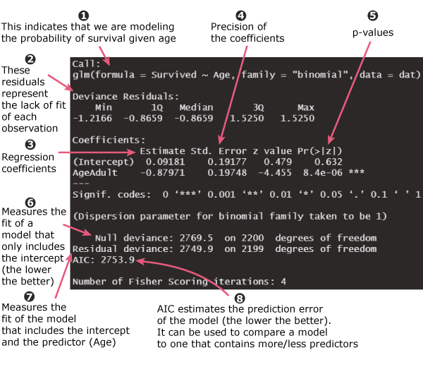
The most critical section is the Coefficients table. The Estimate here is not the change in the outcome itself, but the change in the log-odds of the outcome for a one-unit increase in the predictor.
- Intercept: The log-odds of the outcome when all predictors in the model are equal to zero.
- Predictor
Estimate: For a one-unit increase in the predictor, the log-odds of the outcome change by this amount, holding other predictors constant.- A positive coefficient means the log-odds increase, making the outcome event more likely.
- A negative coefficient means the log-odds decrease, making the outcome event less likely.
This short clip from the "StatQuest with Josh Starmer" channel gives a great explanation of this core concept.
Logistic Regression in R, Clearly Explained!!!!
This StatQuest video excels at explaining the meaning of the coefficients in a logistic regression model.
Watch the segment from interpreting coefficients. The speaker clearly explains how the intercept represents the log-odds for the reference group (females, in his example) and how the predictor's coefficient represents the change in log-odds (the log-odds ratio).
For a more detailed walkthrough that aligns with your interest in medical research, the following resource is excellent.
Chapter 33 Logistic Regression and Broom for Tidying Models
This chapter from "Reproducible Medical Research with R" provides a practical guide to fitting and interpreting glm() models in a medical context. We will focus on the initial model fitting and summary interpretation.
First, read the introductory section that starts just below the chapter title and ends before "The Model Summary". It shows how to fit a model using glm(). Then, carefully read the breakdown of the initial output, focusing on the explanations for coefficients, deviance, and AIC. Finally, read the section "33.1 The Model Summary." Pay close attention to the interpretation of the summary() output, especially the explanation of the coefficients table and what a positive versus negative estimate means on the log-odds scale, as discussed here.
A Real-World Research Example
To see how these steps come together in a publication-style analysis, let's look at a paper from the Malawi Medical Journal that investigates predictors of child immunization. You don't need to fit the model yourself right now, but focus on how the authors set up their data and call the glm() function, connecting theory to practice.
A Practical Guide to Key Considerations in Logistic Regression for ...
This paper provides a step-by-step tutorial on using logistic regression in public health research. We will focus on the data setup and model fitting steps.
First, skim the data preparation code under the heading "Data sets analysed". Notice how the authors use dplyr to create a binary outcome variable, full_immunisation, coded as 1 for 'yes' and 0 for 'no'. This is a critical first step. Next, read "Step 1: Define the research question" and the "quick checks" to see how they inspect the outcome distribution. Finally, jump to "Step 4: Model specification." Find the R code where they fit the model and observe the glm() call: mod_linear <- glm(...). You can see the formula notation and the family = binomial argument in action within a real research context.
Conclusion
In this lesson, you've learned the fundamental principles of binomial logistic regression, a critical tool for analyzing the binary outcomes that are ubiquitous in clinical and health research. You now understand why and when to use it over linear regression and have mastered the R syntax for fitting a model.
Key Takeaways:
- Logistic regression is used for binary outcomes (e.g., yes/no, present/absent).
- It works by modeling the log-odds (logit) of the outcome as a linear combination of the predictors.
- In R, you fit these models with the
glm()function, using thefamily = "binomial"argument. - The coefficients (
Estimate) in thesummary()output represent the change in the log-odds of the outcome for a one-unit change in the predictor. - A positive coefficient increases the log-odds (and probability) of the event, while a negative coefficient decreases it.
Preview of the Next Lesson:
While understanding log-odds is crucial for grasping how the model works, it's not a very intuitive scale for communicating results to clinicians, patients, or policymakers. In our next lesson, we will focus on the essential skill of converting these log-odds coefficients into Odds Ratios (ORs). Odds ratios are the standard way of reporting logistic regression results in medical literature, and mastering their interpretation is key to producing publication-quality analysis.