Variables and Basic Data Types

Introduction

In our last session, you successfully installed and loaded the tidyverse package, giving you access to a powerful suite of data analysis tools. This was a crucial step in setting up your R environment.

Now that you have your tools ready, it's time to start programming. This lesson marks your first real step into writing R code. We will cover how to assign values to variables and how to identify R's basic data types: numeric, character, and logical.

Understanding these concepts is the absolute foundation of all programming. Every analysis you perform, from summarizing patient demographics to fitting complex statistical models, begins with storing data in variables of the correct type.

1. What are Variables? Storing Your Data

Think of a variable as a labeled box where you can store a piece of information. Instead of writing the information on a scrap of paper that you might lose, you put it in the box and give it a clear, descriptive name. In R, you can then refer to the information just by using the box's name.

To create a variable, you need three things:

1. A name for your variable.
2. The assignment operator, which is <-. You can type this as a "less-than" sign followed by a hyphen. It tells R to "put the thing on the right into the object on the left."
3. The value you want to store.

For example, to store a patient's age, you could write:

patient_age <- 42

Now, whenever you want to use the number 42, you can just use the variable name patient_age.

This short video demonstrates this fundamental concept of assigning values to variables.

Naming Your Variables

Choosing good names for your variables is a critical skill. patient_age is much more informative than x. R has a few rules for naming variables.

To summarize the key naming rules from the reading:

• Variable names can contain letters, numbers, dots (.), and underscores (_).
• They cannot start with a number or an underscore.
• They cannot contain spaces or hyphens.
• Names are case-sensitive (patient_age is different from Patient_Age).
• A common convention is to use snake_case, where you separate words with an underscore (e.g., baseline_heart_rate).

2. The Core Data Types

The value you store in a variable has a type. This is crucial because the type determines what you can do with the variable. For example, it makes sense to do math on numbers, but it doesn't make sense to try to multiply two names together.

Let's explore this with a very practical example.

As the reading shows, R must know the type of data you're giving it. The three most fundamental data types you'll use constantly are:

• numeric: For numbers. This includes integers (like 10) and decimals (like 37.5). You write them directly.

  patient_weight_kg <- 85.5
  number_of_doses <- 3
  

• character: For text, also known as "strings". This includes names, categories, or any other non-numeric information. You must enclose character values in quotation marks (" or ').

  treatment_group <- "Drug A"
  patient_id <- "PID-007"
  

• logical: For true or false values. This is essential for checks and comparisons. There are only two possible logical values: TRUE and FALSE. You must write them in all caps and without quotes.

  is_smoker <- TRUE
  has_completed_treatment <- FALSE
  

This video from DataCamp provides a clear, narrated overview of these three data types.

3. How to Check a Variable's Type

As your analyses become more complex, you'll sometimes need to check what type of data is stored in a variable. This is a common debugging step. The easiest way to do this is with the class() function.

You simply put the name of your variable inside the parentheses:

# Create some variables
patient_age <- 42
treatment_group <- "Drug A"
is_smoker <- TRUE




# Check their class
class(patient_age)



# [1] "numeric"

class(treatment_group)



# [1] "character"

class(is_smoker)



# [1] "logical"

The DataCamp video you just watched introduced this function at the beginning (00:06-00:30), and it's a tool you will use frequently.

Let's Practice

Now it's time to apply what you've learned.

1. Open your clinical-trial-practice project in RStudio.
2. If it's not already open, open your 01-analysis.R script from the scripts folder.
3. Below your library() calls, add a new comment like # --- Variable Assignments --- to keep your script organized.
4. Below this comment, create the following variables representing data for a fictional participant. Choose appropriate variable names using the snake_case convention.
   • A patient ID: "P012"
   • The patient's age in years: 54
   • The patient's baseline systolic blood pressure: 145.8
   • A value indicating whether the patient is in the placebo group: TRUE
5. After creating the variables, use the class() function to check the data type of each one.
6. Run each line of your code by placing your cursor on it and pressing Ctrl+Enter (or Cmd+Return on Mac). Observe the output in your console.

Your script might look something like this:

# --- Variable Assignments ---




# 1. Create variables for a participant
patient_id <- "P012"
age_in_years <- 54
baseline_sbp <- 145.8
is_placebo_group <- TRUE




# 2. Check the class of each variable
class(patient_id)
class(age_in_years)
class(baseline_sbp)
class(is_placebo_group)

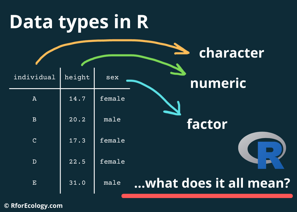
This simple infographic provides a great summary of the data types you've learned about today, plus a few others you'll encounter later.

Conclusion

Excellent work! You've just mastered the first and most fundamental building blocks of R programming. You can now create variables to store information and you understand the difference between numbers, text, and logical values.

Key Takeaways:

• You store information in variables using the assignment operator <-.
• Variable names should be descriptive and follow R's naming rules (e.g., snake_case, no spaces).
• The three core data types are:
  • numeric: For numbers (no quotes).
  • character: For text (must be in quotes).
  • logical: For TRUE or FALSE values (all caps, no quotes).
• You can always check a variable's type with the class() function.

Preview of the Next Lesson:
Now that you know how to store data, the next logical step is to learn how to operate on it. In our next lesson, we will cover arithmetic, comparison, and logical operators. You will learn how to perform calculations (+, -), make comparisons (>, ==), and combine logical conditions (&, |) to start answering basic questions with your data.