Operators: Arithmetic, Comparison, and Logical

Introduction

In the previous lesson, you learned how to store single pieces of information—like a patient's age or treatment group—into variables using R's basic data types: numeric, character, and logical.

Now that you know how to store data, it's time to learn how to operate on it. This lesson focuses on the fundamental actions you can perform with your variables. We will cover how to perform arithmetic, comparison, and logical operations.

Specifically, you will learn to:

• Use arithmetic operators (+, -, *, /, ^) to perform calculations.
• Use comparison operators (==, !=, >, <) to ask true-or-false questions about your data.
• Use logical operators (&, |, !) to combine those true-or-false conditions into more complex queries.

Mastering these operators is essential. They are the verbs of the R language, allowing you to move from simply storing data to actively analyzing it—for instance, calculating a Body Mass Index (BMI), checking if a lab value is outside a normal range, or identifying participants who meet multiple criteria for a study subgroup.

1. Arithmetic Operators: R as a Calculator

At its most basic level, you can use R just like a powerful calculator. You can perform calculations on numbers directly or, more usefully, on the numeric variables you've created.

The standard arithmetic operators are likely familiar to you. Let's start with a foundational reading that covers these operators and the crucial concept of "order of operations."

As you read, the key takeaways are:

• Addition: +
• Subtraction: -
• Multiplication: *
• Division: /
• Exponentiation (Power): ^

The order of operations (often remembered by acronyms like BEDMAS or PEMDAS) is critical:

1. Brackets ()
2. Exponents ^
3. Division / and Multiplication * (from left to right)
4. Addition + and Subtraction - (from left to right)

For example, let's calculate the BMI for a patient who is 1.75 meters tall and weighs 70 kilograms. The formula is $\text{weight}/{\text{height}}^2$.

patient_weight_kg <- 70
patient_height_m <- 1.75




# Calculate BMI
bmi <- patient_weight_kg / patient_height_m^2



# R first calculates patient_height_m^2 (1.75^2 = 3.0625)
# Then it performs the division: 70 / 3.0625




# Print the result
bmi



# [1] 22.85714

If we didn't respect the order of operations and used parentheses incorrectly, we would get the wrong answer.

Now, let's watch a practical demonstration of these operators being used in RStudio.

2. Comparison Operators: Asking Questions

Comparison operators allow you to compare two values. The result of a comparison is always a logical value: TRUE or FALSE. This is how you start to ask analytical questions, such as "Is this patient's blood pressure above the threshold?"

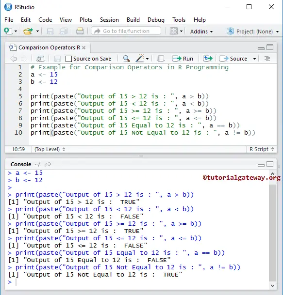
The main comparison operators are:

• == : is equal to (Note the double equals sign!)
• != : is not equal to
• > : is greater than
• < : is less than
• >=: is greater than or equal to
• <=: is less than or equal to

Let's use our bmi variable from before. Suppose a clinical guideline defines "overweight" as a BMI of 25 or greater. We can check if our patient meets this criterion:

is_overweight <- bmi >= 25
is_overweight



# [1] FALSE

The variable is_overweight now holds the logical value FALSE.

An Important Note on Comparing Numbers

When working with decimal numbers that result from calculations, using == can sometimes be unreliable due to the way computers store them. Tiny, invisible rounding differences can make two numbers that look identical appear different to R.

For now, just be aware of this issue. For most of your work, == will be fine, but if you get unexpected FALSE results when comparing calculated numbers, dplyr::near() is the tool to use.

3. Logical Operators: Combining Conditions

Often, you need to check if multiple conditions are true. This is where logical operators come in. They work on logical values (TRUE/FALSE) to produce a new logical value.

• & : AND - returns TRUE only if conditions on both sides are true.
• | : OR - returns TRUE if the condition on either side (or both) is true.
• ! : NOT - reverses a logical value (!TRUE becomes FALSE, and !FALSE becomes TRUE).

This next video gives a fantastic, clear explanation of these three operators.

Let's apply this. Imagine we're screening for patients who might be at high risk: they are over 60 years old AND have a systolic blood pressure over 140.

patient_age <- 65
patient_sbp <- 142

high_risk <- patient_age > 60 & patient_sbp > 140
high_risk



# [1] TRUE
# Both conditions are true, so the result is TRUE.

patient_age <- 55
patient_sbp <- 142

high_risk <- patient_age > 60 & patient_sbp > 140
high_risk



# [1] FALSE
# The first condition is false, so the result is FALSE.

Now, what if the criteria were "over 60 OR blood pressure over 140"?

# Using the second patient
high_risk <- patient_age > 60 | patient_sbp > 140
high_risk



# [1] TRUE
# The second condition (patient_sbp > 140) is true, so the result is TRUE.

A More Efficient "OR": The %in% Operator

A very common task is to check if a value is one of several possibilities. For instance, checking if a patient is in "Group A" or "Group B" or "Group C". You could write group == "A" | group == "B" | group == "C", but this gets tedious.

A much better way is to use the %in% operator. It checks if a value on the left is present in a collection of values on the right.

Here's an example related to your goals:

# Suppose we have three active treatment arms
active_groups <- c("Drug A", "Drug B", "High Dose")




# Check which patients are in any active treatment group
patient_1_group <- "Drug A"
patient_2_group <- "Placebo"

patient_1_group %in% active_groups



# [1] TRUE

patient_2_group %in% active_groups



# [1] FALSE

This is much cleaner and easier to read.

Let's Practice

Time to put all these operators together.

1. In your clinical-trial-practice RStudio Project, open your 01-analysis.R script.
2. Add a new comment section: # --- Operators Practice ---.
3. Create variables for a new patient:
   • participant_id <- "P045"
   • age <- 68
   • treatment_group <- "Placebo"
   • baseline_glucose_mg_dl <- 128 (Glucose in mg/dL)
4. Perform calculations:
   • The normal range for glucose is often cited in mmol/L. To convert mg/dL to mmol/L, you divide by 18.018. Create a new variable baseline_glucose_mmol_l with the converted value.
5. Perform comparisons:
   • A glucose level above 7.0 mmol/L is often a threshold for high blood sugar. Create a variable is_high_glucose that checks if baseline_glucose_mmol_l is greater than 7.0.
   • A participant is considered "older" if their age is 65 or greater. Create a variable is_older_participant.
6. Combine conditions:
   • We want to identify older participants in the placebo group who have high glucose. Create a variable meets_criteria_for_followup that is TRUE only if all three conditions are met:
     1. is_older_participant is TRUE.
     2. treatment_group is equal to "Placebo".
     3. is_high_glucose is TRUE.
7. Use the print() function to display the value of your final variable, meets_criteria_for_followup. Run your code to see the result.

Take your time to write the code for each step. Your solution will involve using arithmetic, comparison, and logical operators.

Conclusion

Great job! You have now learned how to use R's fundamental operators to perform calculations and ask logical questions of your data. This is a huge step forward from simply storing data.

Key Takeaways:

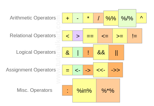
• Arithmetic operators (+, -, *, /, ^) let you perform mathematical calculations. R follows the standard order of operations (BEDMAS/PEMDAS).
• Comparison operators (==, !=, >, <) compare values and always return a logical TRUE or FALSE.
• Logical operators (& for AND, | for OR, ! for NOT) allow you to combine multiple logical conditions to form complex rules.
• The %in% operator is a highly efficient way to check if a value is present within a set of other values.

Preview of the Next Lesson:
So far, we've only operated on single values stored in variables. In real-world data analysis, you'll almost always be working with entire columns of data at once. In the next lesson, we will introduce R's core data structures, starting with vectors. You'll see how the operators you learned today can be applied to whole collections of data simultaneously, which is where R's power for data analysis truly begins to shine.