Importing Data from CSV, Excel, and SPSS Files

Introduction

In our last lesson, you learned how to construct R's primary data structures—vectors, lists, and most importantly, data frames—from scratch. While this is essential for understanding how R organizes information, in your day-to-day work as a researcher, you will rarely type out your data by hand. Your data will already exist in files, perhaps exported from a lab instrument, a patient database, or shared by a collaborator.

This lesson focuses on the crucial next step: bringing that external data into your R environment. You will learn how to import data from CSV, Excel, and SPSS files. These are three of the most common formats you'll encounter in clinical and academic research. We'll use a suite of powerful packages from the Tidyverse—readr, readxl, and haven—to make this process smooth and reliable. Mastering data import is the gateway to analyzing real-world datasets.

1. The Universal Standard: Importing CSV Files with readr

The simplest and most robust format for storing rectangular data is the Comma-Separated Values (.csv) file. A CSV is a plain text file where columns are separated by commas and rows are separated by new lines. Because of its simplicity, it can be opened by almost any data analysis software, making it a universal standard for sharing data.

The readr package, part of the core tidyverse, is R's primary tool for reading plain text data files. Its main function for this task is read_csv().

Let's see how it works.

As you saw in the reading, the basic syntax is straightforward: my_data <- read_csv("path/to/your/file.csv").

A Helping Hand: RStudio's Import GUI

RStudio provides a helpful graphical user interface (GUI) for importing data, which is great for learning because it shows you the code it's generating. In the "Environment" pane (top-right), you can click "Import Dataset" -> "From Text (readr)...".

Handling Messy CSV Files

Real-world data is often messy. You might receive files with introductory text before the actual data starts, or files without proper column headers. read_csv() has arguments to handle this. Two of the most common are:

• skip = n: Tells R to skip the first n lines of the file.
• col_names = FALSE: Tells R that the first row is not a header, but actual data. R will then assign default names (X1, X2, etc.).

2. The Ubiquitous Spreadsheet: Importing Excel Files with readxl

In clinical settings, it's extremely common for data to be collected and stored in Microsoft Excel spreadsheets (.xls or .xlsx). While Excel is a flexible tool, this flexibility can lead to data that is difficult to import programmatically. You might find merged cells, multiple tables on one sheet, titles and notes mixed in with data, or data spread across multiple sheets.

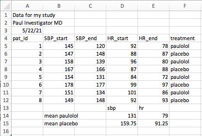
The readxl package is designed to handle these challenges. It reads Excel files directly without any external dependencies like Java, making it highly reliable.

As the video showed, the key function is read_excel(). Its most important arguments for cleaning up messy files are:

• sheet = "SheetName" or sheet = 2: Specifies which sheet to read, either by its name or its position. By default, it only reads the first one.
• skip = n: Just like with read_csv(), this skips the first n rows. This is essential for files like the one pictured above.
• n_max = n: Tells R to read only n rows of data after skipping. This is useful for ignoring summary rows at the bottom of a sheet.

Let's see how these arguments can be used to import the messy paulolol.xlsx file.

3. Collaborating with Colleagues: Importing SPSS Files with haven

SPSS is a statistical software package that has been a mainstay in medical, social, and health sciences for decades. It is highly probable that you will need to work with data from collaborators who use SPSS. These files typically have a .sav extension.

The haven package is the Tidyverse solution for importing data from other statistical packages, including SPSS, Stata, and SAS. A major advantage of haven is that it preserves valuable metadata. For example, SPSS uses "value labels" (e.g., the number 1 might be labeled as "Male" and 2 as "Female"). haven imports these as a special type of vector that retains both the number and the label, which is incredibly useful.

The function for importing SPSS files is haven::read_sav(). As with the other import functions, you simply provide the path to the file.

# First, you might need to install the package if you haven't already
# install.packages("haven")







# Then, load it and use the function
library(haven)
my_spss_data <- read_sav("path/to/your/file.sav")

The haven package is a bridge that allows you, an R user, to seamlessly collaborate with colleagues using other statistical software, a vital skill for interdisciplinary research.

Let's Practice

It's time to apply these skills. In your clinical-trial-practice RStudio Project:

1. Create a new R Script file and save it as 02-data-import.R.
2. At the top of the script, add comments with your name and the date, and a title for the script.
3. Install necessary packages. If you have already installed the tidyverse package, you have readr and readxl. You may still need haven. Add this code to your script and run it. It's okay to run install.packages() on a package you already have.

   
   
   
   
   
   
   # Install packages if needed
   install.packages("tidyverse") # Includes readr and readxl
   install.packages("haven")
   
   
   
   
   
   
   
   # Load the packages for this session
   library(tidyverse)
   library(haven)
   

4. Task 1: Import a CSV file. The palmerpenguins dataset is a modern alternative to the classic iris dataset. Import it directly from its URL.

   
   
   
   
   
   
   # Task 1: Import penguins data from a CSV URL
   penguins_url <- "https://raw.githubusercontent.com/allisonhorst/palmerpenguins/main/inst/extdata/penguins.csv"
   penguins_data <- read_csv(penguins_url)
   
   
   
   
   
   
   
   # Inspect the first few lines
   print(penguins_data)
   

5. Task 2: Import from a messy Excel file. Using the paulolol.xlsx file from our lesson, import only the clean, rectangular patient data. You will need to use the skip and n_max arguments correctly.

   
   
   
   
   
   
   # Task 2: Import from a messy Excel file
   clinical_url <- "https://github.com/higgi13425/rmrwr-book/raw/master/data/paulolol.xlsx"
   clinical_data <- read_excel(clinical_url, skip = 3, n_max = 8) # Hint: Check the lesson for the right numbers!
   
   
   
   
   
   
   
   # Inspect the imported data
   print(clinical_data)
   

6. Task 3: Import an SPSS file. This dataset is from a historical clinical trial on the use of streptomycin for tuberculosis. Import it from its URL.

   
   
   
   
   
   
   # Task 3: Import an SPSS data file
   tb_url <- "https://raw.githubusercontent.com/higgi13425/rmrwr-book/master/data/strep_tb.sav"
   tb_data <- read_sav(tb_url)
   
   
   
   
   
   
   
   # Inspect the imported data
   print(tb_data)
   

Run each chunk of code in your script. In your Environment pane, you should now see three new data frames: penguins_data, clinical_data, and tb_data.

Conclusion

You have just acquired a fundamental skill for any data analyst: getting data into your workspace. You've seen that while the goal is always to have a clean, rectangular data frame, the path to get there requires knowing the right tools and their options.

Key Takeaways:

• readr::read_csv(): The standard for importing data from .csv files. It's fast, reliable, and forms the foundation of data import.
• readxl::read_excel(): Your tool for the inevitable task of reading data from Excel files. Its sheet, skip, and n_max arguments are essential for taming messy spreadsheets.
• haven::read_sav(): The bridge to collaborating with colleagues using SPSS (and other statistical packages). It handles specific metadata like value labels gracefully.
• Problem-Solving: Data import is often the first step in data cleaning. Learning to use function arguments to solve import issues is a critical skill.

Preview of the Next Lesson:
Now that you have successfully imported several datasets into R, what's next? Before you can analyze or visualize data, you must first understand its structure. In our next lesson, you will learn how to examine the structure of a data frame using str(), glimpse(), and summary(). These functions will become your go-to tools for the initial exploration of any new dataset you encounter.