DataFrame Manipulation with Indexing and Boolean Masking

1. From NumPy Arrays to Pandas DataFrames

At its heart, a Pandas DataFrame is a two-dimensional, size-mutable, and potentially heterogeneous tabular data structure with labeled axes (rows and columns). You can think of it as a supercharged spreadsheet or a SQL table, but with the full power of Python.

Crucially, a DataFrame is built upon NumPy arrays. Each column in a DataFrame is a Pandas Series, which is essentially a one-dimensional labeled array. The data within that Series is stored in a NumPy ndarray. This design choice means that the vectorized operations and broadcasting principles you learned in the last lesson apply directly to operations on Pandas Series and DataFrames, allowing for highly efficient data manipulation.

2. The Pillars of Indexing: .loc and .iloc

To work with data in a DataFrame, you first need to know how to access it. Pandas provides two primary, explicit methods for indexing: .loc and .iloc. Understanding the distinction between them is one of the most important foundational concepts in Pandas.

• .loc[] is label-based. It selects data based on the index labels and column names.
• .iloc[] is integer position-based. It selects data based on its integer position, starting from 0, just like a standard Python list or NumPy array.

This distinction is especially important when it comes to slicing:

• Slicing with .loc is inclusive of both the start and end labels.
• Slicing with .iloc is exclusive of the end position, following Python's convention.

The following image provides a clear visual summary of this core difference.

To see these indexers in action, the following video provides a practical walkthrough using a real-world dataset.

While the video gives a great overview, it's also useful to read through a detailed guide with more code examples. The following article provides a thorough comparison and addresses some common "gotchas," such as when an operation returns a Series versus a DataFrame.

3. Powerful Filtering with Boolean Indexing

Often, you don't want to select data by its position or label, but by its content. For instance, you might want to find all rows where a certain value is above a threshold, or all entries belonging to a specific category. This is achieved using boolean indexing, also known as creating a "mask".

This process directly leverages the vectorized nature of Pandas (and NumPy). When you apply a comparison operator (like ==, >, <) to a Pandas Series, it doesn't return a single True or False. Instead, it performs the comparison element-wise and returns a new Series of boolean values. This boolean Series is your "mask," which you can then use to select rows from your DataFrame.

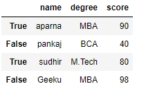
The following video masterfully explains this concept, connecting it directly to the broadcasting principle from our last lesson.

To filter based on multiple conditions, you can combine boolean masks using the bitwise operators & (and) and | (or). Due to Python's operator precedence rules, you must wrap each individual condition in parentheses.

For example: df[(df['age'] > 30) & (df['country'] == 'Canada')]

4. Modifying Data

Once you've mastered selecting data, modifying it is straightforward. You simply use a selection statement on the left side of an assignment operator (=). The recommended and most robust way to do this is with .loc, as it avoids ambiguity and a common warning in Pandas called SettingWithCopyWarning.

You can modify a single cell, an entire column, or a slice of rows and columns. A particularly powerful pattern is to combine boolean indexing with assignment to conditionally update values.

# Create a sample DataFrame
import pandas as pd
data = {'product': ['A', 'B', 'A', 'C', 'B'],
        'price': [100, 150, 110, 200, 140],
        'in_stock': [True, True, False, True, True]}
df = pd.DataFrame(data)




# Example 1: Update the price of a specific product (row 0)
df.loc[0, 'price'] = 105




# Example 2: Apply a 10% discount to all products
df['price'] = df['price'] * 0.9




# Example 3: Mark all products with a price over 120 as "premium"
df.loc[df['price'] > 120, 'category'] = 'premium'

print(df)

The article you read earlier also has a concise section on this technique.

5. A Comprehensive View of Indexing

While .loc and .iloc are the workhorses of Pandas indexing, you've seen a few other methods. It's helpful to have a consolidated view of all the techniques. The resource below provides an excellent chapter on Pandas, including a handy cheatsheet that summarizes all the selection methods.

Conclusion

In this lesson, we transitioned from the raw numerical power of NumPy to the flexible data structures of Pandas. You've learned the essential techniques for accessing and manipulating data within a DataFrame, which is the starting point for nearly every data analysis and machine learning task.

Key takeaways from this lesson:

• DataFrames are built on NumPy, enabling efficient, vectorized operations.
• .loc[] is for label-based selection and uses inclusive slicing.
• .iloc[] is for integer position-based selection and uses exclusive slicing.
• Boolean indexing is a powerful method for filtering data based on its content, by creating a "mask" from one or more conditions.
• Data can be modified by using a selection accessor like .loc[] on the left side of an assignment.

In our next lesson, we will continue our exploration of Pandas by moving from selecting data to transforming it. We will cover aggregation and reshaping operations using powerful tools like groupby, merge, and pivot, which allow you to summarize and restructure your data to uncover deeper insights.