Crafting Publication-Ready Visualizations with Matplotlib and Seaborn

Hello! In our previous lesson, we explored how to aggregate and reshape data using Pandas with groupby, merge, and pivot_table. These powerful tools allow you to transform raw data into a structured format, perfect for analysis. Now, we'll take the next logical step: turning that structured data into insightful, professional-grade visualizations.

This lesson focuses on creating publication-quality plots using two essential Python libraries: Matplotlib and Seaborn. For someone aiming to become an AI Research Engineer, the ability to produce clear, effective, and aesthetically pleasing figures for papers and presentations is not a luxury—it's a core skill. We will cover the fundamental principles that separate a quick, default plot from a polished, publication-ready one. We will start with the fine-grained control offered by Matplotlib and then move to the high-level, statistically-aware plotting capabilities of Seaborn.

1. The Anatomy of a Plot: Matplotlib's Object-Oriented Approach

Before we can create beautiful plots, we must understand how Matplotlib constructs them. While you may have seen simple examples using plt.plot(), this "stateful" approach is less flexible and can be confusing for complex figures. For reproducible, high-quality work, we will use Matplotlib's object-oriented API.

This model has a clear hierarchy:

Figure: The top-level container for everything. It's the overall window or page that everything is drawn on. You can think of it as the canvas.
Axes: This is what you probably think of as 'a plot'. It's the region of the image with the data space, ticks, labels, etc. A single Figure can contain multiple Axes objects (subplots).

The standard way to create a Figure and one or more Axes is with plt.subplots().

import matplotlib.pyplot as plt
import numpy as np




# Create a Figure and a single Axes object
fig, ax = plt.subplots()

x = np.linspace(0, 10, 100)
y = np.sin(x)




# Use the Axes object to plot
ax.plot(x, y)
ax.set_title("A Simple Sine Wave")
ax.set_xlabel("x")
ax.set_ylabel("sin(x)")

plt.show()

By getting a reference to the ax object, we can precisely control every aspect of that specific plot. This object-oriented method is the foundation for all the advanced customization we will perform.

2. Principles of a Publication-Quality Figure

Creating a figure for a research paper involves much more than just visualizing data. It requires a deliberate set of design choices to ensure clarity, readability, and professionalism. A default plot from any library is rarely sufficient.

The following video provides an excellent walkthrough of transforming a standard, "not very beautiful" plot into a polished, research-ready figure. It's a case study that embodies the principles we'll be discussing. As you watch, pay close attention not just to what is changed, but why.

How to Create Beautiful Research Figures (Complete Tutorial)

This tutorial from ChuScience is a masterclass in refining a plot for publication. It systematically identifies the flaws in a default plot and applies targeted improvements.

First, watch the section demonstrating a basic plot with default parameters and the discussion of its numerous problems: creating the default plot and the analysis of its issues. This covers problems with size, resolution, fonts, colors, and legends. Next, follow the step-by-step refinement process. Each step addresses one of the identified issues: Step 1: Plotting Limits - Adjusting the view to focus on the data. Step 2: Fonts - Setting an appropriate font family and size for readability in a manuscript. Step 3: Aspect Ratio & Grids - Enforcing a square plot and adding subtle gridlines. Step 4: Colors - Choosing a deliberate, minimalistic color palette. Step 5: Marker & Line Sizes - Adjusting element sizes for visibility. Step 6: Z-order - Controlling the layering of plot elements. Step 7: Legend - Designing a compact, well-placed legend. Finally, watch the comparison of all the steps to see the dramatic cumulative effect of these changes: revising the steps.

The video provides a fantastic high-level overview. Let's formalize some of those key principles using a more focused resource.

Python Tip: Ready to Publish Matplotlib Figures

This article from Python For The Lab dives into the technical details of setting up a figure for publication, focusing on the critical parameters for size, resolution, and fonts.

Read the sections on Size and DPI. This explains the crucial difference between the physical size of the figure (in inches) and its resolution (in dots per inch). A common standard for print is 600 DPI. Next, read about Font Size. Note that font size is specified in points and relates to the physical figsize, not the DPI. You must set your figsize to what it will be in the final paper first, then choose your font sizes. Finally, review the Saving section. This explains the difference between raster formats (like PNG) and vector formats (like PDF or SVG). For publications, vector formats are almost always preferred because they can be scaled to any size without losing quality.

3. Practical Customization in Matplotlib

With the principles in mind, let's see how to apply them. The following article provides a hands-on guide to customizing line plots, but the techniques apply to most plot types.

Making publication-quality figures in python (Part II): Line ...

This Towards Data Science article gives practical code examples for controlling the appearance of plot elements.

First, read the section on drawing a line plot. Focus on the arguments used to control the plot's appearance: marker, markersize, markerfacecolor, linestyle, and linewidth. Next, review the section on Colors and "zorder". The zorder parameter is particularly important as it controls which elements are drawn on top of others, allowing you to place data points in front of regression lines, for example. Finally, read the section on Legends. Pay attention to the two ways of creating a legend: the simple label argument and the more powerful method of explicitly passing handles and labels to ax.legend(). The latter gives you complete control over the legend's content and appearance.

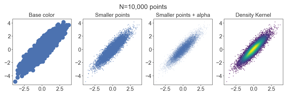
A common challenge, especially in machine learning datasets, is overplotting, where thousands of data points obscure each other. The solution is to adjust marker size and transparency (alpha).

This series of plots shows how reducing marker size and adding transparency (alpha) can reveal the underlying density of a large dataset. A density kernel plot is another effective technique for visualizing dense data.

4. High-Level Statistical Visualization with Seaborn

Matplotlib provides ultimate control, but it can be verbose for complex statistical plots. Seaborn is a library built on top of Matplotlib that provides a high-level API for creating beautiful and informative statistical graphics.

Seaborn's main strength is its deep integration with Pandas DataFrames. It allows you to map columns of your DataFrame to visual properties of the plot, like color (hue), marker style (style), and size (size), often with just a single line of code.

The following video is a crash course that covers the philosophy and a wide range of plots available in Seaborn.

Seaborn Crash Course - Data Visualization in Python

This video from NeuralNine is a fast-paced but thorough introduction to Seaborn.

Start by watching the introduction to understand what Seaborn is and how it relates to Matplotlib. Next, see how to customize the overall look with themes and color palettes. Seaborn comes with several attractive default styles. Watch the core section on plotting, which introduces the key idea of mapping data features to plot aesthetics. Focus on these examples: scatterplot and relplot: Notice how hue, size, and style are used to add dimensions to the plot, and how relplot creates subplots (col). displot, histplot, and kdeplot: For visualizing the distribution of a single variable. catplot (categorical plots): This covers a wide range of useful plots like boxplot, violinplot, and barplot. jointplot and pairplot: Excellent tools for exploring relationships between multiple variables. heatmap: Especially useful for visualizing correlation matrices, a staple of exploratory data analysis. lmplot: Automatically fits and plots a linear regression model.

A typical bar plot created with Seaborn, comparing two methods across three categories. Note the automatic generation of the legend, grouped bars, and error bars, which would require significant manual effort in Matplotlib.

5. Combining the Best of Both Worlds

Because Seaborn is built on Matplotlib, they work together seamlessly. The typical workflow is:

Use Seaborn to quickly create the main statistical plot (e.g., a boxplot or heatmap).
Use Matplotlib's object-oriented API to perform fine-grained customizations that Seaborn might not expose directly (e.g., adding specific annotations, adjusting tick parameters, or changing a title).

Most Seaborn functions return the Matplotlib Axes object, allowing you to immediately start customizing it.

import seaborn as sns
import matplotlib.pyplot as plt

tips = sns.load_dataset("tips")




# 1. Create the plot with Seaborn
fig, ax = plt.subplots(figsize=(8, 6), dpi=100)
sns.scatterplot(data=tips, x="total_bill", y="tip", hue="day", ax=ax)




# 2. Customize with Matplotlib
ax.set_title("Tip Amount vs. Total Bill", fontsize=16)
ax.set_xlabel("Total Bill ($)", fontsize=12)
ax.set_ylabel("Tip ($)", fontsize=12)
ax.legend(title="Day of the Week")

plt.show()

This hybrid approach leverages Seaborn's statistical power and Matplotlib's comprehensive control, enabling you to produce virtually any visualization you need with high efficiency and quality.

Conclusion

In this lesson, we explored the art and science of data visualization for a research context. You've moved beyond simple plotting commands to a principled approach for creating figures that are clear, informative, and professional.

Here are the key takeaways:

Use Matplotlib's Object-Oriented API (fig, ax = plt.subplots()) for full control and reproducibility.
Publication quality is a design process. It requires deliberate choices about figure size (figsize), resolution (dpi), fonts, colors, and the save format (prefer vector formats like PDF/SVG).
Matplotlib is your tool for fine-grained control over every element of a plot.
Seaborn excels at creating complex statistical visualizations quickly by mapping DataFrame columns to visual properties like hue, style, and col.
Combine Seaborn and Matplotlib to get the best of both: rapid generation of statistical plots and detailed final customizations.

In the next lesson, we will dive into preprocessing data for machine learning. The visualization skills you've just learned will be indispensable for inspecting your data before and after applying techniques like handling missing values, encoding categorical features, and feature scaling. Visualizing distributions is often the best way to verify that your preprocessing steps have worked as intended.