NumPy Vectorization and Broadcasting

Welcome to our fourth lesson in the "Python for Data Science and ML" module. In our last session, we constructed our first machine learning models using Python's Object-Oriented Programming features. While this gave our code a clean and reusable structure, you may have noticed that the underlying logic often relied on Python for loops. As we concluded, this approach, while clear, is computationally inefficient and doesn't scale to the massive datasets used in modern machine learning.

Today, we will address this critical performance bottleneck by introducing NumPy, the cornerstone of numerical computing in Python. This lesson focuses on two of its most powerful features: vectorization and broadcasting. You will learn how to replace slow Python loops with highly optimized array operations and how to perform arithmetic on arrays of different shapes. Mastering these concepts is fundamental for implementing performant ML algorithms from scratch, a key skill for any AI research engineer.

1. The Need for Speed: Why Python Loops Are Slow

Before diving into the solution, it's essential to understand the problem. Your background in computer science provides a strong foundation for appreciating the technical reasons behind Python's performance characteristics. Standard Python loops are relatively slow for numerical tasks primarily due to the language's dynamic nature.

Let's explore the core reasons why NumPy is so much faster than native Python code for these operations. The following video provides an excellent conceptual overview.

Vectorization in Python : Data Science Code

Watch this segment from the ritvikmath channel to understand the fundamental principles that make vectorized operations fast.

Watch the first part of the video from the beginning. As you watch, focus on the three key reasons presented for NumPy's speed: Parallelism: How operations can be split across multiple CPU cores. Data Types: The advantage of knowing that an array contains only one type of data (e.g., all float64), which eliminates the per-element type-checking overhead inherent in Python lists. Locality of Reference: How storing data in a contiguous block of memory improves cache performance and data access speed.

To summarize, Python is an interpreted, dynamically-typed language. When it iterates through a list, it must perform type-checking and other overhead for every single element at runtime. In contrast, NumPy pushes these operations down to pre-compiled, highly optimized C code. Because a NumPy array has a fixed data type and is stored in a contiguous block of memory, it can bypass the Python interpreter's overhead and leverage low-level hardware optimizations like SIMD (Single Instruction, Multiple Data) instructions.

2. Vectorization in Practice: From Loops to One-Liners

Vectorization is the process of rewriting loop-based code to use operations on entire arrays at once. This not only makes the code orders of magnitude faster but also more concise and readable.

Let's see this in action. The same video provides a compelling demonstration of the performance difference between a Python loop and a vectorized NumPy operation for both simple element-wise addition and a more complex matrix multiplication task.

Vectorization in Python : Data Science Code

This part of the video provides concrete code examples and benchmarks that quantify the incredible speedup from vectorization.

First, watch the demonstration of element-wise addition. Note the dramatic difference in both code complexity and execution time between the for loop and the simple x + y syntax with NumPy arrays. Next, observe the even more stark contrast in the matrix multiplication example. A triply-nested loop is replaced by a single call to np.dot(), resulting in a speedup of over 7500x.

This massive performance gain is the reason why nearly all ML, deep learning, and scientific computing libraries in Python (like Pandas, Scikit-learn, PyTorch, and TensorFlow) are built on top of NumPy. When you implement an algorithm, your goal should always be to "vectorize" it—express the computations in terms of array operations rather than explicit loops over elements.

3. Broadcasting: Arithmetic on Mismatched Shapes

Vectorization is straightforward when arrays have the same shape. But what happens if you want to add a scalar to a vector, or add a column vector to each column of a matrix? This is where broadcasting comes in.

Broadcasting describes how NumPy treats arrays with different shapes during arithmetic operations. Subject to certain constraints, the smaller array is "broadcast" across the larger array so that they have compatible shapes. This is a powerful feature that allows for vectorized operations in a wider range of scenarios.

The following article gives a clear introduction to this idea.

NumPy Optimization: Vectorization and Broadcasting

This article introduces the concept of broadcasting with a practical example.

Read the section titled Broadcasting. Pay attention to the example of adding a column vector to a matrix. The author first shows a loop-based approach, then a "column-stacking" approach, before introducing broadcasting as NumPy's elegant and efficient solution.

This process is highly efficient because NumPy doesn't actually create copies of the smaller array in memory. It's a conceptual "stretching" that is handled at a lower level by manipulating how the array's data is traversed, which we'll touch on later.

This image illustrates three broadcasting scenarios. Top: A scalar is broadcast to match a 1D array. Middle: A 1D array is broadcast to match a 2D array by being duplicated across rows. Bottom: A column vector (shape 3,1) and a row vector (shape 1,3) are both broadcast to create a 3x3 result.

4. The Rules of Broadcasting

For broadcasting to work, the shapes of the two arrays must be compatible according to a strict set of rules. Understanding these rules is crucial for predicting the behavior of your code and debugging shape-related errors, which are common when implementing ML algorithms.

The video below from the mCoding channel provides a crystal-clear explanation of these rules and then offers an invaluable conceptual model for understanding how NumPy computes the result.

Numpy Array Broadcasting In Python Explained

This video breaks down the rules of broadcasting and then explains the underlying logic using a for-loop analogy, which will resonate with your programming background.

First, watch the segment on the rules of compatibility. The two key rules are: Rule 1: The shapes are right-aligned. If one shape is shorter, it is padded with 1s on the left. For example, when comparing an array of shape (4, 3) with one of shape (3,), the latter is treated as (1, 3). Rule 2: When comparing dimensions from right to left, they are compatible if they are equal, or if one of them is 1. Next, watch the segment explaining how the operation is computed. The presenter uses a brilliant analogy of nested for loops to show how NumPy conceptually fills the output array. This demystifies the process, showing that when an array has a dimension of size 1, its index for that dimension is always treated as 0 during the operation.

Let's formalize the rules:
When operating on two arrays, NumPy compares their shapes element-wise, starting from the trailing (rightmost) dimensions.

Rank alignment: If the two arrays have different numbers of dimensions (different ranks), the shape of the one with fewer dimensions is padded with ones on its leading (left) side.
Dimension compatibility: Two dimensions are compatible if:
- they are equal, or
- one of them is 1.
Error condition: If these conditions are not met for all dimension pairs, a ValueError is raised, indicating the arrays are not broadcast-compatible.
Output shape: The shape of the resulting array is the element-wise maximum of the two input array shapes.

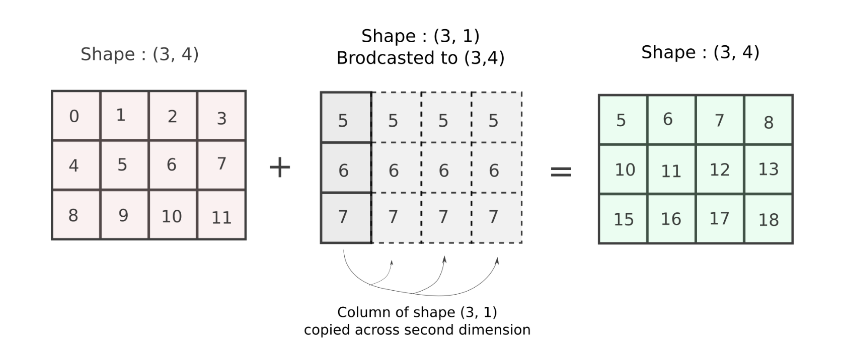
Let's walk through an example: A.shape = (3, 1) and B.shape = (3, 4).

The shapes are (3, 1) and (3, 4).
Comparing the rightmost dimensions: 1 and 4. They are compatible because one is 1. The resulting dimension size is max(1, 4) = 4.
Comparing the next dimensions: 3 and 3. They are compatible because they are equal. The resulting dimension size is max(3, 3) = 3.
The final output shape is (3, 4).

Here, a column vector of shape (3, 1) is added to a matrix of shape (3, 4). The column vector is broadcast across the second dimension to match the (3, 4) shape, enabling an element-wise addition.

5. How Broadcasting Really Works: A Glimpse into Strides

You might be wondering how NumPy achieves broadcasting without making "needless copies of data." The answer lies in a low-level concept called strides. This will be particularly interesting given your systems-level knowledge from your CS studies.

An array's data is stored in a contiguous 1D block of memory. The array's metadata includes its shape and its strides. A stride is a tuple that specifies the number of bytes to jump in memory to get to the next element along each dimension.

Broadcasting works by cleverly manipulating these strides. When a dimension of size 1 is broadcast to a larger size, the corresponding stride for that dimension is set to 0. This means that as NumPy iterates along that broadcasted dimension, it doesn't move its memory pointer at all—it simply re-reads the same data. This creates a "virtual" larger array without consuming any extra memory.

The following article provides a more detailed explanation of this mechanism.

Advanced NumPy Broadcasting and Strides Guide - Analytics Vidhya

This article explains the underlying mechanism of strides that makes broadcasting memory-efficient.

Read the section Broadcasting and Strides in NumPy. Focus on understanding the definition of a stride and how a stride of 0 allows an array to be virtually expanded without copying data. The example showing how to repeat a row vector using as_strided and a 0 stride is a powerful illustration of this principle.

While you won't typically manipulate strides directly, understanding that they are the mechanism behind broadcasting provides a complete mental model of how NumPy achieves its remarkable efficiency.

Conclusion

In this lesson, we moved from the slow, explicit loops of native Python to the high-speed world of vectorized computing with NumPy. This is a foundational shift in thinking that is essential for performance-critical work in AI and data science.

Here are the key takeaways:

Vectorization is the practice of replacing element-by-element loops with operations applied to entire arrays, yielding massive speedups by leveraging compiled code and low-level hardware optimizations.
Broadcasting extends the power of vectorization by providing a clear set of rules for performing arithmetic on arrays with different but compatible shapes.
Broadcasting is extremely memory-efficient, as it avoids creating copies of data by manipulating array strides to create "virtual" arrays.

You are now equipped with the fundamental tools for high-performance numerical computation in Python. In our next lesson, we will build directly upon this foundation as we explore Pandas, the premier library for working with tabular data. You'll see how the NumPy arrays we've studied today form the underlying data structure for Pandas DataFrames, and you'll learn how to select, filter, and modify data within these powerful structures.