Choropleth Maps: Visualizing Violation Rates

What is a Choropleth Map?

Before we start coding, let's clarify what we're building. A choropleth map is a thematic map where areas are shaded or patterned in proportion to a statistical variable. For your project, the areas are districts or states, and the statistical variable is the meal quality violation rate you've calculated.

This technique is exceptionally powerful for revealing spatial patterns that are difficult to discern from tables of numbers alone.

Creating Your First Map with GeoPandas

Given your experience with pandas and Matplotlib, you'll find GeoPandas' plotting functionality quite intuitive. The primary method we'll use is .plot(), which is an extension of the pandas plotting method, but designed for geographic data.

The most critical parameter for creating a choropleth map is column. You pass the name of the column in your GeoDataFrame that contains the numerical data you want to visualize. In your case, this will be the violation_rate column.

The following resource, which uses an India-based dataset, provides a complete walkthrough. While we covered the data merging part in the last lesson, its plotting section is now our main focus.

A basic plot command would look something like this, assuming your merged data is in a variable named merged_gdf:

import matplotlib.pyplot as plt




# Create a figure and axes
fig, ax = plt.subplots(1, 1, figsize=(10, 10))




# Plot the choropleth map
merged_gdf.plot(column='violation_rate', 
                ax=ax, 
                legend=True)




# Show the plot
plt.show()

Polishing Your Visualization

The basic plot is functional, but to create a map that is clear, professional, and ready for your final report, you'll need to customize it. This involves choosing appropriate colors, styling the legend, adding a title, and removing distracting elements like axis ticks.

This video provides an excellent visual demonstration of how to transform a default plot into a polished map.

Here is a summary of the key customization parameters you'll use:

• cmap: Specifies the color map. Choosing an effective color map is crucial for clear communication. Sequential colormaps (e.g., 'OrRd', 'Blues') are great for data that goes from low to high. Diverging colormaps (e.g., 'RdBu') are useful for showing deviations from a central value.
• legend=True: Enables the color bar legend.
• legend_kwds: A dictionary of keywords to customize the legend. Common keys include label (to title the legend), orientation ('horizontal' or 'vertical'), and shrink (to control its size).
• edgecolor: The color of the borders between geographic regions. A subtle color like '0.8' (light grey) is often effective.
• linewidth: The thickness of the region borders.
• missing_kwds: A dictionary to style regions that have no data. This is useful for making it clear which areas are missing data versus which have low values.

An Important Consideration: Normalizing Data

A common pitfall in choropleth mapping is visualizing raw counts (e.g., total number of complaints) instead of rates (e.g., complaints per 1000 people). Raw counts often just map population density, as more populous areas naturally have more events.

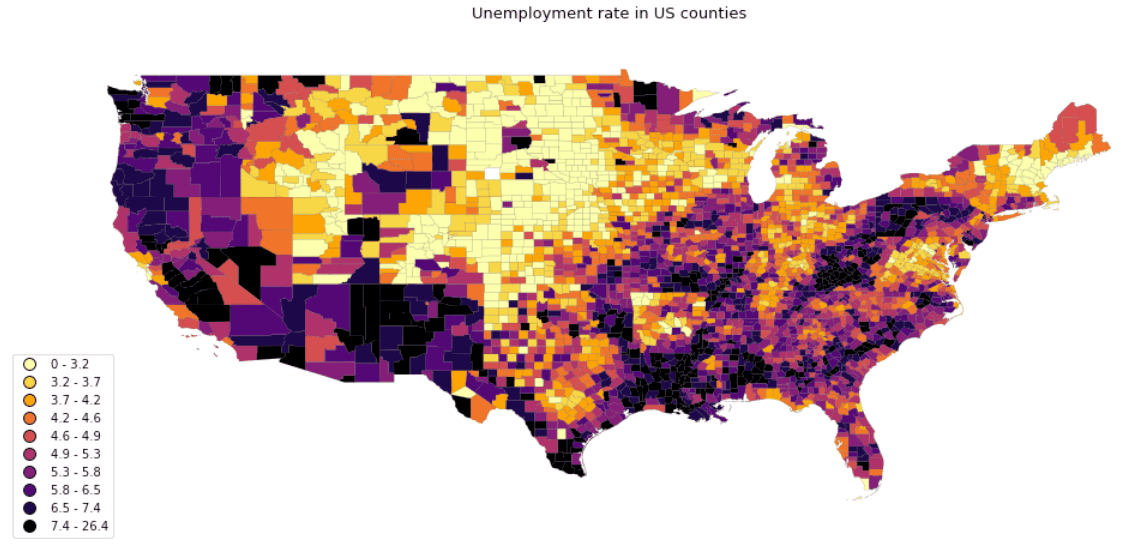
Since you are calculating a violation_rate, you are already performing this normalization. However, your data might still be heavily skewed, with a few regions having extremely high violation rates (outliers) and most having low rates. This can result in a map where most regions are the same light color, and only one or two are dark, hiding the variation in the lower-range values.

The following resource explains this problem and a common solution: using a logarithmic scale.

If you find your map lacks detail, you can apply a log transformation to your violation_rate column before plotting. This compresses the range of the high-end outliers and expands the range of the low-end values, often resulting in a much more nuanced and informative visualization.

import numpy as np




# Apply a log10 transformation
# Add a small constant to avoid log(0) errors if rates can be zero
merged_gdf['log_violation_rate'] = np.log10(merged_gdf['violation_rate'] + 0.01)




# ... then plot the 'log_violation_rate' column

Bringing It All Together

Here's a complete code block that incorporates these concepts to generate a polished choropleth map for your project. You can adapt this as a template.

import geopandas as gpd
import matplotlib.pyplot as plt
import numpy as np




# Assume 'merged_gdf' is your GeoDataFrame from the previous lesson
# It has a 'geometry' column and a 'violation_rate' column




# --- Data Preparation for Visualization ---
# Handle missing data if any, e.g., fill with a specific value or drop
merged_gdf['violation_rate'].fillna(0, inplace=True)




# Optional: Apply log transformation if data is heavily skewed
# merged_gdf['plot_variable'] = np.log10(merged_gdf['violation_rate'] + 0.01) 
merged_gdf['plot_variable'] = merged_gdf['violation_rate'] # Or use the raw rate




# --- Plotting ---
fig, ax = plt.subplots(1, 1, figsize=(12, 12))




# Remove axis ticks and labels for a cleaner look
ax.set_axis_off()




# Add a title
ax.set_title('Midday Meal Violation Rates by District', fontdict={'fontsize': '16', 'fontweight': '3'})




# Plot the choropleth map
merged_gdf.plot(column='plot_variable',
                cmap='OrRd',          # Choose a color map
                linewidth=0.8,
                ax=ax,
                edgecolor='0.8',     # Light grey for borders
                legend=True,
                legend_kwds={'label': "Violation Rate",
                             'orientation': "horizontal",
                             'shrink': 0.6},
                missing_kwds={"color": "lightgrey",
                              "label": "Missing values"}
                )




# Save the figure
plt.savefig("violation_hotspot_map.png", dpi=300)

plt.show()

Finally, to save your map for your report, you can use the savefig method from Matplotlib, as shown in the code above and in the final step of the Medium article.

Conclusion

In this lesson, you have learned how to take your processed geospatial data and turn it into a compelling and informative choropleth map. This is a cornerstone of geospatial analysis, enabling you to communicate complex spatial patterns effectively.

Key takeaways include:

• Choropleth maps visualize statistical data across geographic regions using color.
• GeoPandas' .plot() method, with the column parameter, is the primary tool for creating these maps.
• Customization is essential for clarity. You can control colors (cmap), borders (edgecolor), legends (legend, legend_kwds), and titles to create a professional-grade visualization.
• For skewed data, visualizing rates over raw counts and applying transformations like a logarithmic scale can reveal more nuanced patterns.

You can now visually identify potential "hotspots" of meal quality violations. However, are these clusters a real pattern, or just random chance? In our next lesson, we will move from visualization to statistical validation by exploring spatial autocorrelation, a method to formally test whether the patterns you see on your map are statistically significant.