In the last lesson, you transformed your raw violation rate data into a powerful choropleth map, giving you a first visual look at the potential geographic hotspots for midday meal quality issues. While these maps are insightful, they beg a critical question: are the clusters you see—for example, a group of districts with high violation rates—a genuine, statistically significant pattern, or could they have occurred simply by random chance?
This lesson introduces the core concept needed to answer that question: spatial autocorrelation. We will explore what it means for data to be "spatially autocorrelated" and why understanding this concept is fundamental to your project's goal of identifying non-random hotspots. This provides the conceptual foundation for the statistical tests we will perform in the subsequent lessons.
The First Law of Geography
At its heart, spatial autocorrelation is a simple, intuitive idea, famously summarized by geographer Waldo Tobler as the "First Law of Geography":
"Everything is related to everything else, but near things are more related than distant things."
For your project, this might mean that a school district with a high violation rate is more likely to be located next to another district with a high violation rate than one with a low rate. Spatial autocorrelation is the formal measure of this tendency.
To understand this concept more deeply, it's helpful to start with a video that breaks down the idea of correlation, auto-correlation (correlation with itself), and finally, spatial auto-correlation.
Spatial Autocorrelation - GeoHero
This short video from GeoHero provides a clear and concise introduction to the topic.
Watch the first minute of the video, the definition, where the presenter explains the concept using an easy-to-understand temperature example.
Types of Spatial Autocorrelation
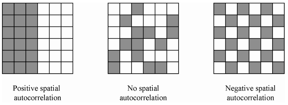
The world isn't always so neatly organized. The opposite of a discernible pattern is spatial randomness, where the value at any given location gives you no information about the values of its neighbors. In a spatially random world, a district with a high violation rate is just as likely to be next to a low-violation district as it is to be next to another high-violation one.
When we test for spatial autocorrelation, our starting assumption (our null hypothesis) is that the data is spatially random. Our goal is to find enough evidence to reject this assumption and prove that a meaningful spatial structure exists.
If we reject randomness, we typically find one of two types of patterns:
-
Positive Spatial Autocorrelation: This is the pattern of clustering. Similar values are located near each other. This is the most common pattern in social and economic data. For your project, finding positive spatial autocorrelation would mean you have identified statistically significant hotspots (clusters of high violation rates) and coldspots (clusters of low violation rates).
-
Negative Spatial Autocorrelation: This is a pattern of dispersion or a "checkerboard" effect. High values tend to be located next to low values, and vice versa. This pattern is less common but might occur in situations of competition, like rival supermarket chains intentionally placing stores away from each other.
The image below provides a simple, abstract illustration of these three possibilities.
For a more formal introduction to these concepts, the following reading from a textbook on Geographic Data Science is excellent.
Global Spatial Autocorrelation — Geographic Data Science with Python
This resource from Geographic Data Science with Python provides a clear, academic definition of spatial autocorrelation and its different forms.
First, read the introductory section The notion of spatial autocorrelation for a formal definition. Then, read the section on understanding the concept. Focus on the definitions of spatial randomness, positive autocorrelation, and negative autocorrelation.
Why Is This Important for Your Project?
Understanding spatial autocorrelation is critical for two main reasons.
First, and most obviously, it is the tool for identifying hotspots. Your choropleth map shows visual clusters. Spatial autocorrelation statistics will tell you whether those clusters are "real" in a statistical sense. This moves your analysis from subjective observation ("it looks like there's a cluster here") to objective proof ("the districts in this region show statistically significant positive spatial autocorrelation").
Second, it validates your statistical approach. Most standard statistical methods you've encountered in your data science coursework (like linear regression) assume that observations are independent of each other. The presence of spatial autocorrelation violates this assumption. If you ignore it, your models might produce misleading results. For example, a model might overstate the importance of a particular variable simply because that variable is itself spatially clustered.
Spatial Autocorrelation - GeoHero
The GeoHero video continues by explaining the practical implications of spatial autocorrelation in modeling.
Watch from importance in modeling. Pay attention to the discussion of "independent observations" and how failing to account for spatial patterns can lead to models that don't generalize well. The example from species distribution modeling at the end is a great illustration of how this can lead to incorrect conclusions.
Ultimately, patterns on a map are often the visible signatures of underlying real-world processes. A hotspot of meal quality violations isn't just a statistical anomaly; it might signal a systemic issue like a single corrupt food supplier for a whole region, a lack of administrative oversight in a particular state, or shared socio-economic factors. Analyzing spatial patterns allows you to form hypotheses about these root causes.
How Does Spatial Autocorrelation Work?
This article frames the importance of spatial autocorrelation as a way to understand the processes that create the patterns we see.
Read the sections titled First Law of Spatial Pattern and Second Law of Spatial Pattern. This reinforces the statistical implications and connects the concept to uncovering why the data is distributed the way it is.
The Building Blocks of a Spatial Autocorrelation Statistic
As we've established, simply looking at a map is not enough because the human brain is wired to see patterns, even in random noise. We need a formal statistic. While we will cover the specific formulas in the next lesson, it's crucial to understand conceptually what such a statistic must do.
Any spatial autocorrelation statistic must combine two distinct pieces of information for every pair of locations in your dataset:
- Attribute Similarity: How similar are the values at location i and location j? For your project, this means comparing the
violation_ratein district i to theviolation_ratein district j. Are they both high? Both low? Or is one high and one low? - Locational Similarity: How "close" are location i and location j? This doesn't just mean geographic distance. It's often defined by a spatial weights matrix, which formally specifies which locations are considered "neighbors." For example, we might define two districts as neighbors if they share a border.
A statistic for spatial autocorrelation, then, essentially calculates a score that reflects the attribute similarity for all pairs of locations that are defined as neighbors.
This complex lecture excerpt from Luc Anselin, a pioneer in this field, explains this fundamental point very clearly.
Week 4a: Spatial autocorrelation (Introduction to Spatial Data Science)
This video from the GeoDa Software channel explains the conceptual construction of a spatial autocorrelation statistic.
Watch the key segment from how to build a statistic. Don't worry about the formulas. Focus on the core idea that a statistic must combine attribute similarity (e.g., are crime rates similar) with locational similarity (are the locations neighbors). This is the conceptual leap from just looking at a map to calculating a formal measure.
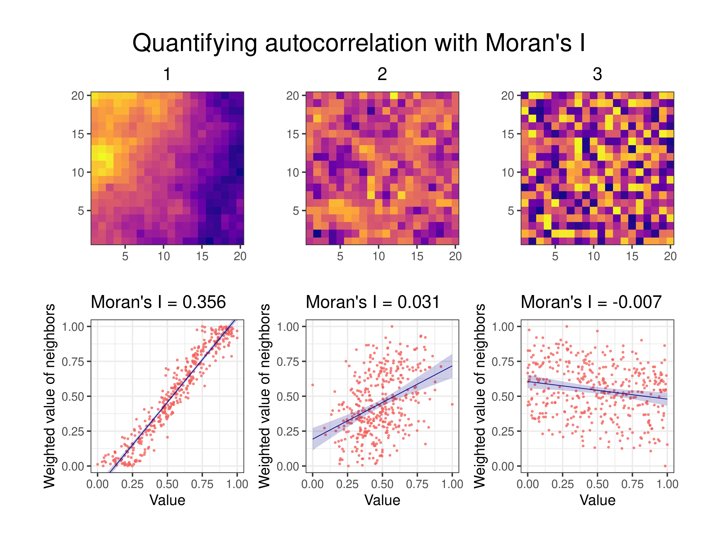
The image below gives a fantastic visual summary of this idea. The heatmaps show the spatial distribution of values, while the scatter plots visualize the relationship between a location's value (x-axis) and the average value of its neighbors (y-axis).
Conclusion
In this lesson, you've moved from visual pattern recognition to a formal understanding of spatial structure. You now have the conceptual tools to interpret the geographic patterns in your data not as random occurrences, but as potential evidence of underlying systemic issues.
Here are the key takeaways:
- Spatial autocorrelation is the measure of how similar values are at nearby locations, summarized by Tobler's Law: "near things are more related than distant things."
- The main types are positive (clustering), negative (dispersion), and zero (spatial randomness). Your search for "hotspots" is a search for significant positive spatial autocorrelation.
- Identifying spatial autocorrelation is crucial for your project because it provides statistical proof of non-random patterns and is necessary to meet the independence assumptions of many models.
- A spatial autocorrelation statistic works by combining a measure of attribute similarity (how similar are the values?) with locational similarity (how close are the locations?).
Now that you understand the what and the why, the next lesson will focus on the how. We will introduce and compute Moran's I, the most common statistic for measuring global spatial autocorrelation, to finally answer the question: are the clusters on your map statistically significant?