Welcome back. In our previous lesson, we explored how top-k and nucleus sampling allow us to control the quality and diversity of generated text by intelligently truncating the model's output distribution. These strategies address what token to pick next. Now, we will turn our attention to the efficiency of this process.
This lesson focuses on a cornerstone of modern LLM inference: KV Caching. You know from your experience with DevOps and software development that redundant computation is a primary enemy of performance. Autoregressive text generation, where each new token depends on all previous ones, is particularly susceptible to this. We will explore how KV caching eliminates a massive source of this redundancy, transforming the computational complexity of generation from quadratic to linear and making real-time applications feasible.
By the end of this lesson, you will be able to explain what KV caching is, how it avoids redundant computation of key and value states, and understand the crucial trade-off it introduces between speed and memory.
The Inefficiency of Naive Autoregressive Generation
Let's begin by understanding the problem that KV caching solves. In an autoregressive model, generating a sequence of text happens one token at a time. To generate token , the model must process all preceding tokens . To generate token , it must process all tokens . This sequential dependency is computationally expensive.
The core of this expense lies within the self-attention mechanism, which, as we've learned, calculates the relevance between tokens using Queries, Keys, and Values. The video below provides a concise overview of the problem and the high-level solution.
KV Cache: The Trick That Makes LLMs Faster
The video "KV Cache: The Trick That Makes LLMs Faster" from Tales Of Tensors introduces the core challenge of quadratic computational growth in autoregressive generation.
Watch from the beginning to the end of the main explanation. Focus on the visualization of how the number of computations grows with each new token and how caching previously computed key and value matrices can break this quadratic scaling.
As the video highlights, the fundamental issue is re-computation. When generating the -th token, the model re-calculates the Key and Value vectors for all the preceding tokens ( through ), even though these tokens and the model's projection weights haven't changed.
Let's formalize this. Recall from our lessons on attention that the Key () and Value () matrices are derived by projecting the input embeddings () with learned weight matrices ( and ):
At inference time, and are fixed. This means that for a given input token embedding , its corresponding key vector and value vector will always be the same, regardless of which future token we are trying to predict. Naively re-running the attention mechanism at every step means wastefully re-computing these identical vectors again and again.
This article provides an excellent, in-depth explanation of this redundancy.
KV Cache Explained: Efficient Attention for LLM Generation ...
This article by Martin Brenndörfer is a comprehensive guide to KV caching. We will use it as our primary reference for this lesson.
Please read the section "The Redundancy Problem in Autoregressive Generation." Pay close attention to the step-by-step trace of how wasted work accumulates and the formula that illustrates the quadratic scaling of projection operations.
The Solution: Caching Keys and Values
The solution, as you've likely inferred, is to compute the Key and Value vectors for each token only once and store them in a cache. This is the essence of KV Caching.
The generation process is split into two phases:
- Prefill (or Prompt Processing): The model processes the entire input prompt in a single, parallel forward pass. It computes the Key and Value vectors for every token in the prompt and stores them in the cache.
- Decode (or Generation): For each new token to be generated, the model only needs to compute the Query, Key, and Value vectors for the single, most recently generated token. It then appends this new Key-Value pair to the cache and computes attention using its new Query vector against the entire cache of Keys and Values.
This is not an approximation; the result is mathematically identical to the naive approach. We are simply avoiding redundant work.
This diagram brilliantly illustrates the core insight.
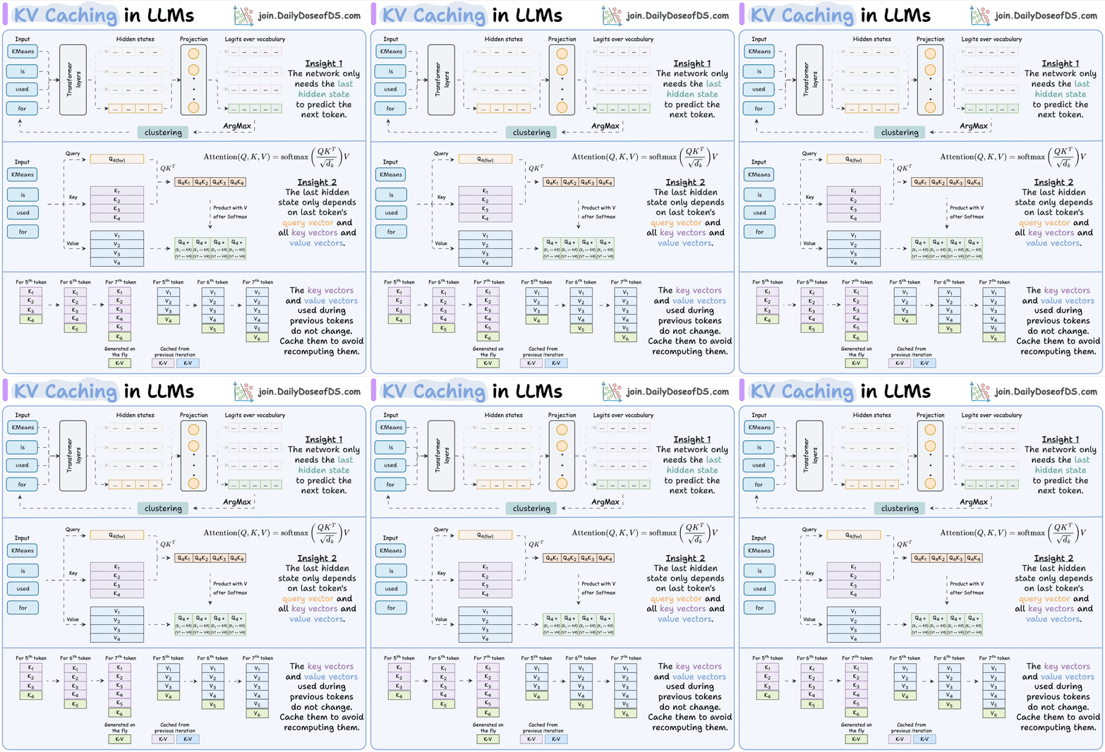
A natural question arises: why don't we cache the Query vectors as well? A token's Query vector represents its "question" about the context at a specific point in the generation. The Query from token is used to attend to tokens . The Query from token will be used to attend to tokens . Since the context it attends to changes and grows, the query's role is unique to each step. It is computed, used immediately to produce the attention output for that step, and can then be discarded. In contrast, the Keys and Values represent the "information content" of each token, which remains constant for all subsequent steps to refer back to.
The following resource formalizes this caching mechanism and provides a complete numerical example.
KV Cache Explained: Efficient Attention for LLM Generation ...
We'll continue with the same article to formalize the solution.
First, read the section "The KV Cache Solution", focusing on the mathematical formulation that distinguishes between the prefill and decode phases. Then, walk through the "Worked Example" section. You don't need to verify every number, but trace the logic: see how projections are computed for all three prompt tokens in the prefill phase, and then for only one new token in the decode phase. This makes the computational savings concrete.
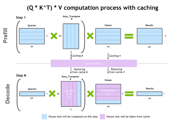
The difference between the prefill and decode steps is also clearly visible in the shapes of the matrices involved.
The Cost of Speed: Memory Consumption
KV caching provides a dramatic speedup, but it comes at a cost: memory. As a DevOps lead, you're accustomed to analyzing resource trade-offs, and this is a classic one. The cache, which stores the Key and Value vectors for every token in the sequence, for every attention head, in every layer, can become enormous.
The total memory required for the cache can be calculated with the following formula:
Cache Size (bytes) = 2 × (Number of Layers) × (Number of Heads) × (Head Dimension) × (Sequence Length) × (Bytes per Parameter)
Let's simplify this. Since d_model = Number of Heads × Head Dimension, the formula becomes:
Cache Size (bytes) = 2 × (Number of Layers) × d_model × (Sequence Length) × (Bytes per Parameter)
This formula reveals a critical point: the cache size scales linearly with the sequence length. For very long contexts or large batch sizes, the KV cache can consume more GPU VRAM than the model weights themselves.
KV Cache Explained: Efficient Attention for LLM Generation ...
Let's analyze the memory implications with our reference article.
Read the sections "Cache Structure" and "Cache Memory Requirements." The concrete calculation for the LLaMA 2 7B model will give you a tangible sense of the memory footprint.
This memory consumption is not just a capacity problem; it creates a performance bottleneck. The decode phase becomes memory-bandwidth-bound. The GPU's powerful arithmetic units are often idle, waiting for the massive KV cache to be loaded from the GPU's high-bandwidth memory (HBM) into the much faster on-chip SRAM for computation. The ratio of computation (FLOPs) to data movement (bytes) is very low, a property known as low arithmetic intensity. Therefore, the speed of inference during the decode phase is often limited not by how fast the GPU can do math, but by how fast it can move the KV cache.
This makes the cache size a primary constraint on system throughput (how many users can be served concurrently) and maximum context length.
Conclusion
In this lesson, we dissected KV caching, the fundamental optimization that makes autoregressive LLM inference practical. By identifying and eliminating redundant computations within the attention mechanism, it reduces the complexity from quadratic to linear with respect to sequence length.
Here are the key takeaways:
- Naive autoregressive generation is inefficient because it repeatedly re-computes Key and Value vectors for tokens that have already been processed.
- KV caching solves this by storing these Key and Value vectors in memory. At each step, only the K and V vectors for the newest token are computed and appended to the cache.
- This optimization is mathematically exact, not an approximation. It changes the computational path but yields an identical result.
- The trade-off is speed for memory. The cache can consume a significant amount of VRAM, scaling linearly with sequence length, model depth, and model width.
- During decoding, inference becomes memory-bandwidth-bound, where the bottleneck is the time taken to move the cache from HBM to SRAM, a scenario of low arithmetic intensity.
The memory cost of the KV cache is such a critical factor that it has motivated a wealth of subsequent architectural innovations and system-level optimizations. In future lessons, we will encounter techniques like Multi-Query Attention (MQA), Grouped-Query Attention (GQA), and PagedAttention, all of which are designed to manage or reduce the size and impact of the KV cache.
Our next module will explore advanced architectural innovations, where we will see some of these cache-reducing techniques in action.