Top-K and Nucleus Sampling: Balancing Diversity and Coherence

The Problem of the Long Tail

When an LLM generates the next token, it produces a probability distribution across its entire vocabulary, which can contain tens of thousands of tokens. While a few tokens might be highly probable, the vast majority have infinitesimal probabilities. Pure sampling from this full distribution, as discussed in the paper "The Curious Case of Neural Text DeGeneration," can lead to incoherent text because the cumulative probability of this "unreliable tail" is non-trivial, making it possible to sample strange or irrelevant tokens.

To mitigate this, we can employ strategies that truncate the distribution before sampling. The most straightforward of these is top-k sampling.

Top-k Sampling: A Fixed-Size Window

Top-k sampling imposes a simple, hard constraint: at each step, we consider only the $k$ most probable tokens for the next word. All other tokens are discarded.

The process is as follows:

1. The model generates logits and computes a probability distribution over the entire vocabulary.
2. The tokens are sorted by their probability in descending order.
3. Only the top $k$ tokens are kept, forming a new, smaller candidate set.
4. The probabilities of these $k$ tokens are renormalized so that they sum to 1.
5. The next token is sampled from this new, smaller distribution.

The following video provides a clear, step-by-step example of this process.

The parameter $k$ provides a direct lever to control the trade-off between diversity and coherence.

• A small $k$ (e.g., 5 or 10) creates a more deterministic and coherent output, as it restricts the model to only the most likely choices.
• A large $k$ (e.g., 100) allows for more diversity and creativity, but risks including less plausible tokens from the distribution's shoulder, potentially reducing coherence.

However, a fixed k is not always optimal. Consider the difference between predicting the next word in these two contexts:

1. "The capital of France is..." (The distribution is sharply peaked around "Paris").
2. "The main character of the story was..." (The distribution is flat across thousands of possible names and descriptions).

In the first case, a small k is ideal. In the second, a small k would stifle creativity by cutting off many reasonable options. This limitation of a static window size is the primary motivation for our next technique: nucleus sampling.

Nucleus (Top-p) Sampling: A Dynamic Window

Instead of selecting a fixed number of tokens, nucleus (or top-p) sampling selects a fixed probability mass. It forms a "nucleus" of the most probable tokens whose cumulative probability exceeds a threshold $p$.

The process, illustrated beautifully in the following diagram, is:

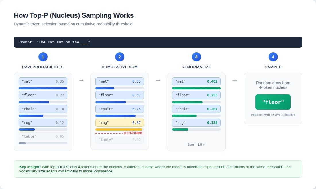
As you can see, the key steps are:

1. Sort tokens by probability.
2. Calculate the cumulative probability from most likely to least likely.
3. Identify the smallest set of tokens for which this cumulative probability is greater than or equal to $p$. This is the nucleus.
4. Renormalize the probabilities of the tokens within the nucleus.
5. Sample from this renormalized distribution.

The crucial advantage is that the size of the nucleus is dynamic.

• For a peaked distribution (high model confidence), only a few tokens are needed to reach the p threshold, resulting in a small, focused candidate set.
• For a flat distribution (low model confidence), many tokens are required to reach p, resulting in a larger, more diverse candidate set.

The original paper that introduced this method provides the formal definition and rationale.

The parameter $p$ typically ranges from 0.9 to 0.99. A value of $p=1.0$ would be equivalent to sampling from the full distribution (with temperature), while a very small $p$ would make the model more deterministic, approaching greedy search.

The following image visually summarizes the difference in how top-k and top-p select their candidate sets.

A Unified View: Decoding as Optimization

So far, we have discussed these sampling methods as a "cookbook" of practical techniques. However, given your background and goals, we can go deeper. A more elegant and fundamental perspective frames decoding as a constrained optimization problem. This view posits that all decoding strategies are implicitly solving the following "Master Problem":

Let's break this down:

• We are choosing an optimal probability distribution $q_t^{\ast }$ over the vocabulary $\mathcal{V}$.
• $⟨q,s_t⟩$ is the expected model score (where $s_t$ are the logits). We want to maximize this.
• $\Omega (q)$ is a regularization term that promotes desirable properties in the distribution, like entropy (diversity). $\lambda$ controls its strength.
• ${\mathcal{C}}_t$ is a constraint set on the support of the distribution $q$.

From this perspective, top-k and top-p are not fundamentally different algorithms. They are solutions to this same master problem, using the same regularizer (negative Shannon entropy), but with different constraints ${\mathcal{C}}_t$.

• Top-k Sampling: The constraint ${\mathcal{C}}_t$ forces the support of $q$ to be the set of the $k$ highest-scoring tokens. It's a fixed-cardinality constraint.
• Top-p Sampling: The constraint ${\mathcal{C}}_t$ forces the support of $q$ to be the nucleus ${\mathcal{V}}_p$. It's a cumulative-mass constraint.

This advanced framing elevates these techniques from mere heuristics to principled solutions of a well-defined optimization problem. A recent paper provides the full derivation.

Conclusion

In this lesson, we have moved from reshaping the full probability distribution with temperature to intelligently truncating it. This allows us to balance diversity and coherence more effectively by focusing only on the most plausible region of the probability space.

Key takeaways from our exploration include:

• Top-k sampling introduces randomness by sampling from a fixed-size set of the $k$ most probable tokens. It is simple but can be too restrictive or too permissive depending on the context.
• Nucleus (top-p) sampling improves upon this by sampling from a dynamic set of tokens whose cumulative probability exceeds a threshold $p$. This allows the candidate set size to adapt to the model's confidence at each step.
• Both methods provide a way to control the trade-off between coherence (by filtering out the noisy tail) and diversity (by sampling from a set of good options).
• From a theoretical standpoint, both can be viewed as solutions to a unified constrained optimization problem, differing only in the nature of the constraint applied to the output distribution's support.

We have now completed our tour of the primary sampling strategies that control the quality of text generation. In our next lesson, we will shift gears from quality to efficiency and explore KV Caching, a crucial optimization that dramatically speeds up the autoregressive generation process.