Token Embeddings: From Discrete IDs to Dense Vectors

From Integers to Vectors: The Embedding Layer

The core component that performs this transformation is the embedding layer. At its heart, an embedding layer is a simple but massive lookup table. This table is a matrix, let's call it $E$, with dimensions $|V|\times d_{\text{embed}}$, where:

• $|V|$ is the size of our vocabulary.
• $d_{\text{embed}}$ is the dimensionality of the embedding vectors, a hyperparameter of the model (e.g., 768 for BERT-base, 12288 for GPT-3).

Each row of this matrix is a vector of length $d_{\text{embed}}$. The process of embedding a token is straightforward: a token with ID i is mapped to the i-th row of the matrix $E$. This row vector is the token's embedding.

From a computational standpoint, this is a highly efficient array-indexing operation. Andrej Karpathy's video provides a clear, practical demonstration of this process in PyTorch.

While we think of this as a direct lookup, it's mathematically equivalent to a linear transformation. Imagine representing a token ID i as a one-hot vector: a vector of length $|V|$ that is all zeros except for a 1 at the i-th position. Multiplying this one-hot vector by the embedding matrix $E$ yields exactly the i-th row of $E$.

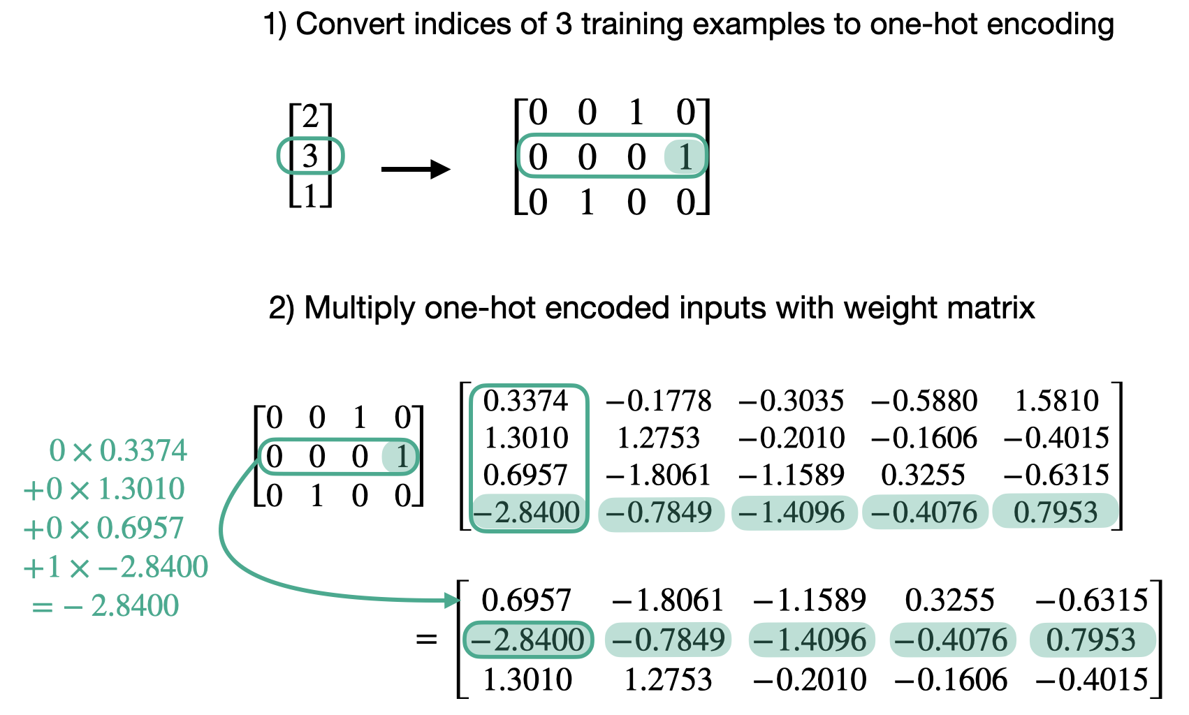
This diagram illustrates the equivalence between one-hot matrix multiplication and a direct lookup. A one-hot vector for token ID '3' (which is [0,0,0,1] if the vocabulary has 4 tokens) is multiplied by the embedding weight matrix. The result is the 4th row of the matrix, which is the embedding for token '3'.

This perspective is powerful because it frames the embedding layer as a linear layer that projects tokens from an extremely high-dimensional, sparse space (where dimensions are equal to the vocabulary size) into a much lower-dimensional, dense vector space. This transition from sparse to dense representation is a cornerstone of modern NLP.

The Geometric Meaning of Embeddings

Why are these dense vectors so special? Unlike one-hot vectors, where every token is equidistant and orthogonal to every other, the vectors in a dense embedding space are learned. The values in the embedding matrix $E$ are model parameters, initialized randomly and then fine-tuned during the training process via backpropagation.

The goal of this learning process is to arrange the vectors in the $d_{\text{embed}}$-dimensional space such that their geometric relationships capture semantic similarities. This is guided by the distributional hypothesis, which posits that words appearing in similar contexts tend to have similar meanings. The training process nudges the vectors of words like "cat" and "dog" closer together, while pushing them further from "car" or "planet".

The result is a rich semantic space where directions correspond to concepts. The 3Blue1Brown channel offers a superb visualization of this phenomenon.

The idea that we can perform arithmetic on word meanings (king - man + woman) is a profound consequence of representing them as vectors in a well-structured space. This structure is not pre-programmed; it is an emergent property learned from statistical patterns in the training data.

How are Semantic Embeddings Learned?

The principles behind learning these embeddings were largely developed in models like Word2Vec, which predated Transformers. While a full derivation is outside our main path, understanding the objective function is insightful, given your background.

A common approach is the skip-gram model. Its objective is, given a center word, to predict the words that appear in its context window. The model contains two embedding matrices (one for center words, one for context words). During training, it adjusts these embedding vectors to maximize the probability of predicting the correct context words.

To formalize this, the model calculates the similarity between the center word vector and all other context word vectors using dot products. These scores are then converted to probabilities using a softmax function. The loss is the negative log-likelihood of the true context words.

For a deeper mathematical treatment, the following article provides a clear breakdown.

In a Transformer, the embedding matrix is simply the first layer of the network, and its weights are learned jointly with all other model parameters to minimize the final language modeling loss. The same principle applies: the gradients flowing back to the embedding layer will adjust the vectors to be more useful for the downstream task of predicting the next token.

Embeddings at the Input and Output: Weight Tying

We've established that the embedding layer maps token IDs to vectors at the model's input. In the previous lesson, we also saw that the final layer of the model, the "unembedding" or language model head, does the reverse: it projects the final hidden state vector into a probability distribution over the entire vocabulary.

This involves a projection matrix of shape $d_{\text{embed}}\times |V|$. Notice the dimensional symmetry with the input embedding matrix, which is $|V|\times d_{\text{embed}}$. This is no coincidence. The intuition is that the vector representation a model uses to understand a token should be the same as the representation it aims to produce when generating that token.

This insight leads to a powerful optimization called weight tying. Instead of learning two separate, massive matrices, we can use a single matrix for both tasks. The output projection matrix is simply the transpose of the input embedding matrix.

Weight tying not only halves the number of parameters in these layers—saving hundreds of millions of parameters in large models—but it also enforces a consistent semantic space throughout the model, often leading to better performance and faster convergence.

Preparing the Input for the Transformer

The token embedding provides the semantic meaning of a token, but it contains no information about its position in the sequence. Because the Transformer processes all tokens in parallel, the raw embeddings for "The dog chased the cat" and "The cat chased the dog" are identical sets of vectors.

To solve this, we must explicitly inject positional information. This is typically done by creating a second vector—a positional embedding—for each position in the sequence and adding it to the corresponding token embedding.

This diagram illustrates the complete input process. After the 'Token Embedding Layer Lookup', the resulting 'Token Embeddings' are combined with 'positional embeddings' to form the final input that is fed into the Transformer's decoder layers.

This combination of semantic and positional information creates the final input representation for the Transformer block.

This crucial topic of how positional embeddings are generated and why they are so vital will be the entire focus of our next lesson.

Conclusion

In this lesson, we have demystified the token embedding layer, the gateway through which text enters the semantic world of a neural network. We've seen that it is much more than a simple conversion utility; it is a learnable component that shapes the very foundation of the model's understanding.

Here are the key takeaways:

• An embedding layer is a lookup table (a matrix of size $|V|\times d_{\text{embed}}$) that maps a discrete token ID to a specific row, which is its dense vector representation.
• This lookup is mathematically equivalent to multiplying a one-hot vector by the embedding matrix, effectively projecting from a sparse, high-dimensional space to a dense, lower-dimensional one.
• The embedding vectors are learned parameters whose geometric arrangement in the vector space captures semantic relationships, enabling conceptual arithmetic (e.g., king - man + woman ≈ queen).
• In Transformers, the input embedding matrix is often tied with the output projection matrix (its transpose), which saves parameters and enforces a consistent semantic representation.
• The final input to the first Transformer block is the sum of the token embedding (what the token means) and a positional embedding (where the token is).

We have now successfully converted our token IDs into meaningful, but position-agnostic, vectors. In the next lesson, we will dive deep into the mathematics of positional encodings, exploring how we can provide the model with the sequential context it needs to understand grammar and long-range dependencies.