Vocabulary and Tokenization in NLP Models

What is a Vocabulary?

In the context of NLP, a vocabulary is the complete, predefined set of all unique tokens a model can process. Think of it as a definitive dictionary. Each token—be it a word, a character, or, as we saw with BPE, a subword—is mapped to a unique integer ID.

This vocabulary is not an inherent property of a language; it is a learned artifact, created during the tokenizer training phase. The vocab_size parameter you might see in tokenizer configurations is a hyperparameter that dictates how many merge operations BPE (or a similar algorithm) will perform, thereby determining the final size of this dictionary.

A typical vocabulary for a modern LLM contains tens of thousands of tokens, including:

• Individual characters or bytes to handle any possible string.
• Commonly occurring subwords (e.g., ing, tion, pre).
• Frequent whole words (e.g., the, and, is).
• Special control tokens (e.g., <|endoftext|>, [CLS], [SEP]).

The tokenization process, therefore, is the act of consulting this vocabulary to convert an input string into a sequence of corresponding integer IDs.

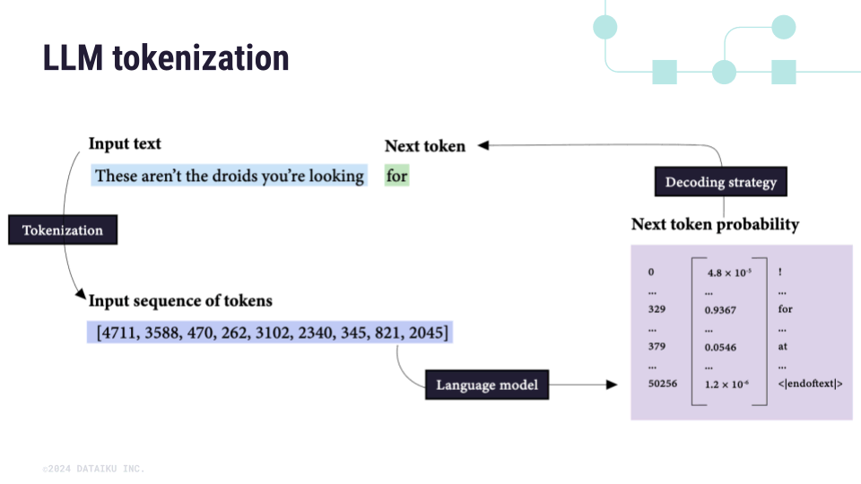
This diagram shows the flow from raw input text to a sequence of integer token IDs. The tokenizer uses its pre-compiled vocabulary to map chunks of text like "for" to their unique ID, in this case, 329.

The Vocabulary's Role at the Model's Input

As established, the vocabulary is the cornerstone of converting text to numbers. But its influence extends directly into the model's architecture. The first layer of a Transformer, the embedding layer, is fundamentally shaped by the vocabulary.

This layer's job is to map the discrete, one-dimensional token IDs into a high-dimensional vector space. It does this using an embedding matrix, a large table of weights. If our vocabulary has a size of $|V|$ and our model's hidden dimension is $d_{\text{model}}$, the embedding matrix will have dimensions $|V|\times d_{\text{model}}$. Each row of this matrix corresponds to a token in the vocabulary and contains its unique vector representation, or "embedding."

The size of this embedding matrix is a significant factor in the total parameter count of a model. For a model like GPT-3 with a vocabulary of ~50,000 tokens and a hidden dimension of 12,288, this single matrix contains over 600 million parameters. This direct relationship between vocabulary size and model size is a critical architectural consideration.

The Vocabulary's Role at the Model's Output

The vocabulary's influence is just as profound at the end of the model as it is at the beginning. An autoregressive language model's fundamental task is to predict the next token in a sequence. This prediction is not a single token but a probability distribution over the entire vocabulary.

To achieve this, the output from the final Transformer layer, which is a vector of dimension $d_{\text{model}}$, must be converted into a vector of dimension $|V|$, where each element represents the likelihood of a corresponding token in the vocabulary. This is accomplished by the language model head, which typically consists of two components:

1. A Linear Layer (Unembedding Layer): This layer projects the final token's output vector from the hidden dimension ($d_{\text{model}}$) up to the vocabulary dimension ($|V|$). This is done by multiplying the vector by an unembedding matrix of shape $d_{\text{model}}\times |V|$. The resulting vector of size $|V|$ contains a raw, unnormalized score for each token in the vocabulary. These scores are called logits.
2. The Softmax Function: The logits are then passed through a softmax function. This function normalizes the scores, converting them into a valid probability distribution where all values are between 0 and 1, and the sum of all values is exactly 1.

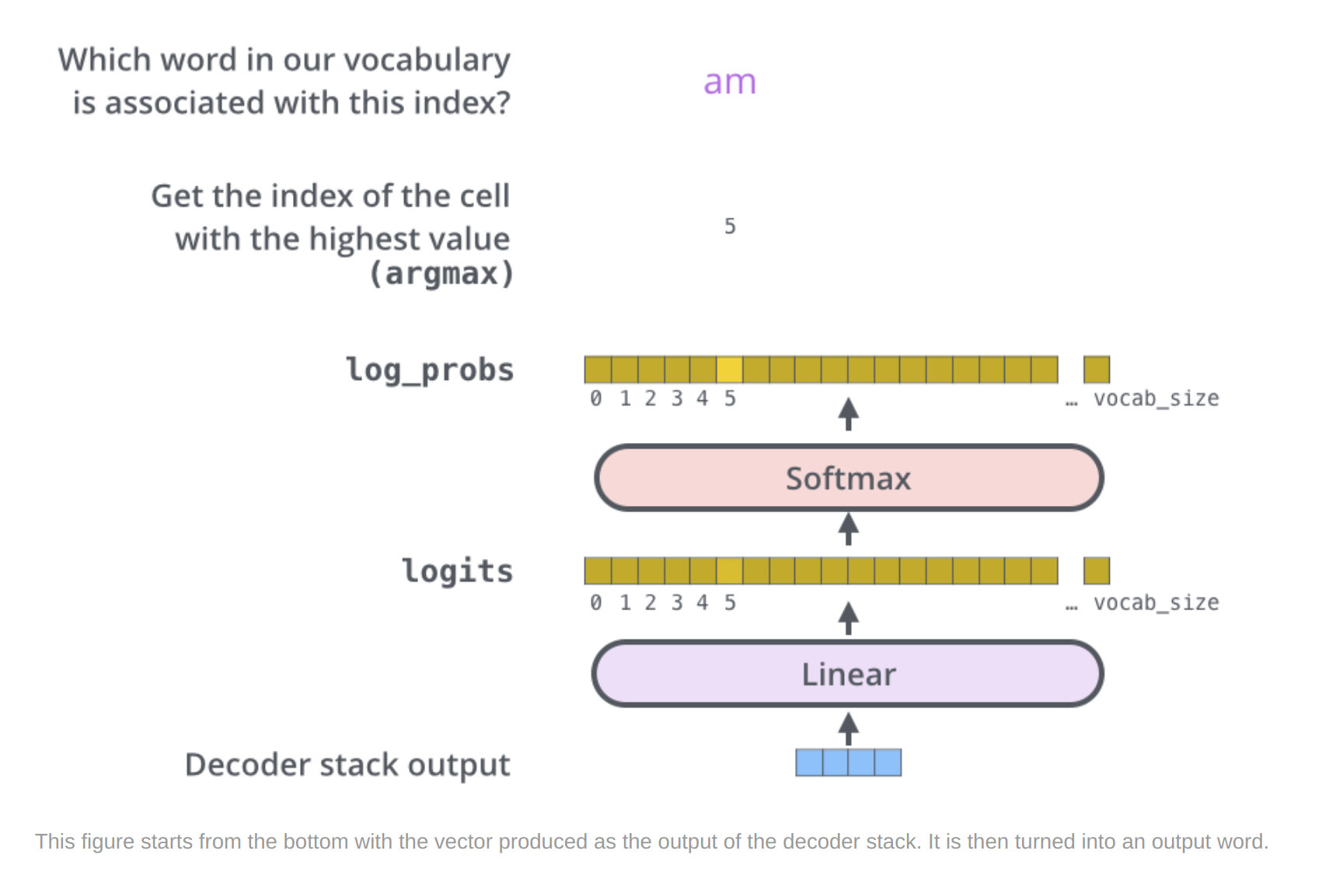
This diagram illustrates the language model head. The Decoder stack output (a vector of size $d_{\text{model}}$) is passed through a Linear layer (the unembedding matrix) to produce logits (a vector of size $|V|$). The Softmax function then converts these logits into log_probs (or probabilities), from which the next token can be sampled.

The following video provides an excellent visual and conceptual walkthrough of this entire output process.

To formalize this, let's turn back to the Jurafsky and Martin text, which provides a precise definition and diagram of the language model head.

The Vocabulary Size Trade-off

Given that the vocabulary size $|V|$ directly determines the size of the input embedding and final output projection matrices, choosing $|V|$ is a critical engineering decision with significant trade-offs.

• A smaller vocabulary results in smaller embedding matrices, reducing the model's memory footprint. However, it forces the tokenizer to break words into more, smaller pieces. This increases the average sequence length ($L$) for a given text, which in turn increases the computational cost of the attention mechanism (which scales with $O(L^2)$).
• A larger vocabulary allows more words to be represented as single tokens, leading to shorter average sequence lengths and reducing the cost of attention. However, it dramatically increases the size of the embedding and unembedding matrices and increases the computational cost of the final softmax layer, which must compute a probability for every token in the vocabulary.

As a computer science student with a background in systems, you can appreciate that this is a classic space-time trade-off, manifesting in the context of neural network architecture.

Conclusion

In this lesson, we have established the central role of the vocabulary in a language model's architecture. It is far more than just a list of tokens; it is a fundamental component that defines the interface between text and the model's numerical world.

Here are the key takeaways:

• The vocabulary is a finite, fixed dictionary mapping all known tokens to unique integer IDs. It is the output of a training process like BPE.
• At the input, the vocabulary size $|V|$ dictates the number of rows in the input embedding matrix ($|V|\times d_{\text{model}}$), a major contributor to the model's total size.
• At the output, the model produces a probability distribution over the entire vocabulary. This requires a language model head consisting of a linear (unembedding) layer to produce logits of size $|V|$ and a softmax function to normalize them into probabilities.
• The choice of vocabulary size involves a critical trade-off between the model's memory/parameter count and the computational cost associated with sequence length and the final softmax calculation.

We have now seen how text is converted to IDs using a vocabulary. The next logical step is to understand what happens in that very first layer of the network. In our next lesson, we will explore token embeddings in detail, examining how these static, high-dimensional vectors are learned and how they manage to capture the rich semantic meaning of language.