Positional Encoding in Transformers

The Problem of Permutation Invariance

Recurrent Neural Networks (RNNs), which preceded Transformers, process sequences token by token. This sequential nature inherently bakes the order of tokens into the computation; the hidden state at step t is a function of the input at t and the hidden state from t-1.

The Transformer, by contrast, was designed to overcome the sequential bottleneck of RNNs and enable massive parallelization. It processes all tokens of an input sequence simultaneously. Its core mechanism, self-attention, calculates the relevance of every token to every other token in the sequence. While powerful, this parallelism creates a new problem: the architecture is permutation-invariant. Without an explicit signal, it has no innate sense of which token came first.

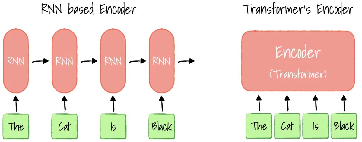
This diagram contrasts the sequential processing of an RNN-based encoder with the parallel processing of a Transformer encoder. The RNN processes tokens one after another, naturally incorporating order. The Transformer processes all tokens at once, requiring an external method to inject positional information.

To truly grasp why this is a deal-breaker, the following video segment explains the issue with a clear example.

Given this, we need a way to "stamp" each token embedding with information about its position.

Naive Approaches and Their Shortcomings

Before diving into the solution, it's instructive to consider simpler ideas and why they fail. Your systems engineering background will appreciate the need for a robust design that satisfies multiple constraints.

1. Integer Indices: Why not just add the token's index (0, 1, 2, ...) to its embedding?

   • Unboundedness: For long sequences, these integer values could become very large, potentially overpowering the semantic information in the token embedding, which is typically initialized with small, normalized values.
   • Generalization: The model might not have seen sequences of a certain length during training, making it difficult to interpret unseen, large position indices.

2. Normalized Indices: What if we normalize the index by the sequence length, so it's always in the range [0, 1]?

   • Inconsistency: The meaning of a position becomes relative. A value of 0.5 would mean the middle token, but this corresponds to position 5 in a 10-token sentence and position 50 in a 100-token sentence. The model cannot learn a consistent meaning for a specific positional offset.

The video segment below discusses these very issues, setting the stage for a more sophisticated solution.

Sinusoidal Positional Encodings: The Formula

The solution presented by Vaswani et al. is to use sine and cosine functions of different frequencies. For a token at position pos and an embedding dimension d_model, the positional encoding vector $PE$ is defined as:

Let's break this down:

• pos is the position of the token in the sequence (e.g., 0, 1, 2, ...).
• i is the dimension index within the embedding vector, ranging from $0$ to $d_{\text{model}}/2-1$. Note that each i corresponds to a pair of dimensions (2i and 2i+1).
• d_model is the dimension of the embeddings (e.g., 768).
• 10000 is a constant chosen by the authors. It determines the range of frequencies.

In essence, each pair of dimensions in the positional encoding vector corresponds to a sinusoid. As the dimension i increases, the term $10000^{2i/d_{\text{model}}}$ grows, which decreases the frequency of the wave.

• For small i (early dimensions), the frequency is high. The values change rapidly with each step in position. These dimensions encode fine-grained, local positional information.
• For large i (later dimensions), the frequency is very low. The values change slowly across the sequence. These dimensions encode coarse, global positional information.

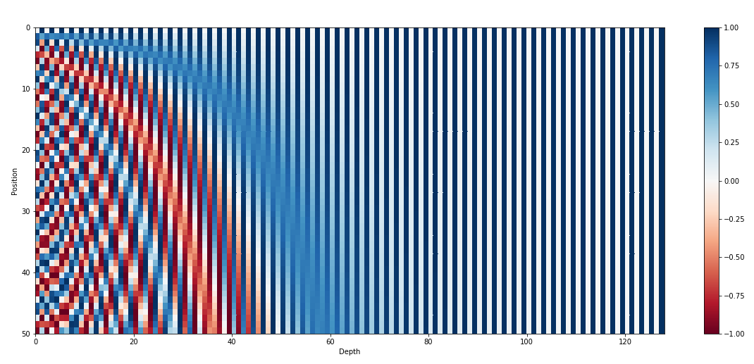
This heatmap visualizes a 128-dimensional positional encoding for the first 50 positions. Each row is a position, and each column is a dimension. You can clearly see the high-frequency oscillations in the early dimensions (left) and the very slow-changing values in the later dimensions (right).

For a more rigorous treatment of the formula and its properties, the following resource is excellent.

The Intuition: From Binary to Continuous Waves

This choice of sinusoids might seem arbitrary, but there is a powerful intuition behind it, which has a nice parallel in computer science: binary representation.

Consider how we represent integers in binary. The least significant bit (LSB) flips at every increment (0, 1, 0, 1, ...). The next bit flips every two increments (0, 0, 1, 1, ...), the next every four, and so on. Each bit position oscillates at a different frequency.

Sinusoidal encodings apply the same principle in a continuous, smooth space. The high-frequency sinusoids are like the LSB, capturing small changes in position, while the low-frequency sinusoids are like the most significant bits, capturing large-scale position. This multi-frequency approach gives every position a unique "fingerprint."

The following video provides an excellent intuitive walkthrough, including the binary analogy and a clever clock-hand analogy to explain how different frequencies capture position at different scales.

The Key Property: Relative Positioning via Linear Transformation

Here lies the mathematical elegance of this method, which is especially powerful. The use of a sin/cos pair for each frequency allows the model to learn about relative positions with remarkable ease.

The core property is that for any fixed offset k, the positional encoding of pos + k can be represented as a linear function (specifically, a 2D rotation) of the positional encoding of pos. The transformation matrix for this rotation depends only on the offset k, not the absolute position pos.

Let's look at a single frequency ${\omega }_i=1/10000^{2i/d_{\text{model}}}$. The positional encoding pair is:

Now consider the encoding for pos + k:

Using the trigonometric angle addition identities:
$\sin (A+B)=\sin (A)\cos (B)+\cos (A)\sin (B)$
$\cos (A+B)=\cos (A)\cos (B)-\sin (A)\sin (B)$

We can rewrite the pos + k vector as a matrix multiplication:

This 2x2 matrix is a standard rotation matrix. Crucially, its elements depend only on the offset k and the frequency ${\omega }_i$, not on pos. This means the relationship between position 5 and 8 is encoded identically to the relationship between position 105 and 108. The self-attention mechanism can learn a single, simple linear transformation to understand concepts like "the token three positions ago."

The Vizuara channel has a fantastic visualization of this rotational property.

For a formal written proof, you can refer back to the article by Amirhossein Kazemnejad.

Conclusion

In this lesson, we have constructed the final input representation for the Transformer. By adding the semantic token embedding to a carefully designed sinusoidal positional encoding, we provide the model with both what a token is and where it is.

Here are the key takeaways from our exploration:

• Necessity: Non-recurrent architectures like the Transformer process tokens in parallel and are permutation-invariant, so positional information must be explicitly injected.
• Design: Sinusoidal encodings solve the shortcomings of naive methods by providing a bounded, deterministic, and unique signal for each position.
• Intuition: The encoding uses a spectrum of frequencies, from high to low, to capture both fine-grained local and coarse-grained global position, analogous to the bits in a binary number.
• Key Property: The pairing of sine and cosine functions for each frequency allows relative positional offsets to be represented as simple linear transformations (rotations). This makes it easy for the attention mechanism to learn patterns based on relative distance.

A final, important point is that this method involves adding the positional encoding to the token embedding. This "mixes" the two signals. While effective, it's not perfect, and this limitation has motivated further research into more advanced techniques like Rotary Positional Embeddings (RoPE), which we will cover in a later module.

Having now fully prepared our input vectors, we are ready to feed them into the heart of the Transformer. In our next lesson, we will begin Module 2 by dissecting the core attention mechanism, exploring how the model uses query, key, and value vectors to dynamically weigh the importance of different tokens in the sequence.