Data Parallelism for Large-Scale Model Training

In our previous lessons, we delved into techniques for optimizing the training process on a single computational device. We learned how gradient accumulation allows us to simulate massive batch sizes and how mixed-precision training cleverly reduces memory footprint and accelerates computation. While powerful, these methods eventually hit the physical limits of a single GPU. To continue scaling our models and datasets, we must transcend the single-device paradigm and orchestrate training across a fleet of processors.

This lesson introduces the most fundamental and widely used multi-device training strategy: data parallelism. Our goal is to describe data parallelism and explain how it enables training on large datasets by replicating the model across multiple devices. We will begin with the foundational concept, explore the communication patterns that make it work, and then progress to the sophisticated, memory-efficient implementations that power modern large-scale training.

Why Go Beyond a Single GPU?

The drive to use multiple devices stems from two primary constraints in deep learning: compute time and memory capacity.

Compute Bottleneck: Training large language models involves processing enormous datasets, often terabytes of text, for many epochs. Even with the fastest available GPU, iterating through such a dataset can take weeks or months. The core motivation for data parallelism is to slash this training time by dividing the computational work of a single large batch across multiple processors simultaneously.
Memory Bottleneck: As we've seen, LLMs have voracious memory appetites. While techniques like mixed precision help, the sheer size of the model parameters, their corresponding gradients, and the optimizer states can easily exceed the memory of a single GPU. Furthermore, even if the model fits, a very large dataset may not.

The following video from Stanford's CS336 course sets the stage by explaining why multi-machine parallelism is an absolute necessity for training state-of-the-art models.

Stanford CS336 Language Modeling from Scratch | Spring 2025 | Lecture 7: Parallelism 1

This clip from the Stanford course on "Parallelism" articulates the core compute and memory challenges that motivate distributed training.

Watch the introductory segment from the beginning. Pay close attention to the distinction between the need for more compute to train models faster and the need to overcome memory limitations as models grow too large to fit on one device.

Data parallelism primarily attacks the compute bottleneck, allowing us to process data much faster. While it doesn't inherently solve the problem of a single model being too large for one GPU, it lays the groundwork for all other parallelization strategies.

The Core Idea: Replicate the Model, Split the Data

Data parallelism operates on a simple and intuitive principle. Instead of processing a large batch of data sequentially on one GPU, we divide the batch into smaller "micro-batches" and process each one on a separate GPU in parallel.

For this to work, each participating device must have a complete copy of the model. The process for a single training step unfolds as follows:

Replication: An identical copy of the model is placed on each of the $N$ available GPUs.
Distribution: A global batch of data is split into $N$ smaller, non-overlapping micro-batches. Each GPU receives one micro-batch.
Parallel Computation: Each GPU independently performs a forward pass with its micro-batch to compute the loss, followed by a backward pass to compute gradients for the model's parameters. At this point, each GPU has a set of gradients derived only from its local data slice.
Synchronization: The gradients from all GPUs are aggregated (typically summed or averaged). This crucial step ensures that the final weight update incorporates information from the entire global batch.
Weight Update: Each GPU uses the synchronized gradients to update its local copy of the model's weights. Because every GPU starts with the same weights and applies the exact same update, the models on all GPUs remain identical, ready for the next iteration.

This workflow is beautifully illustrated in the following diagram for a two-node setup.

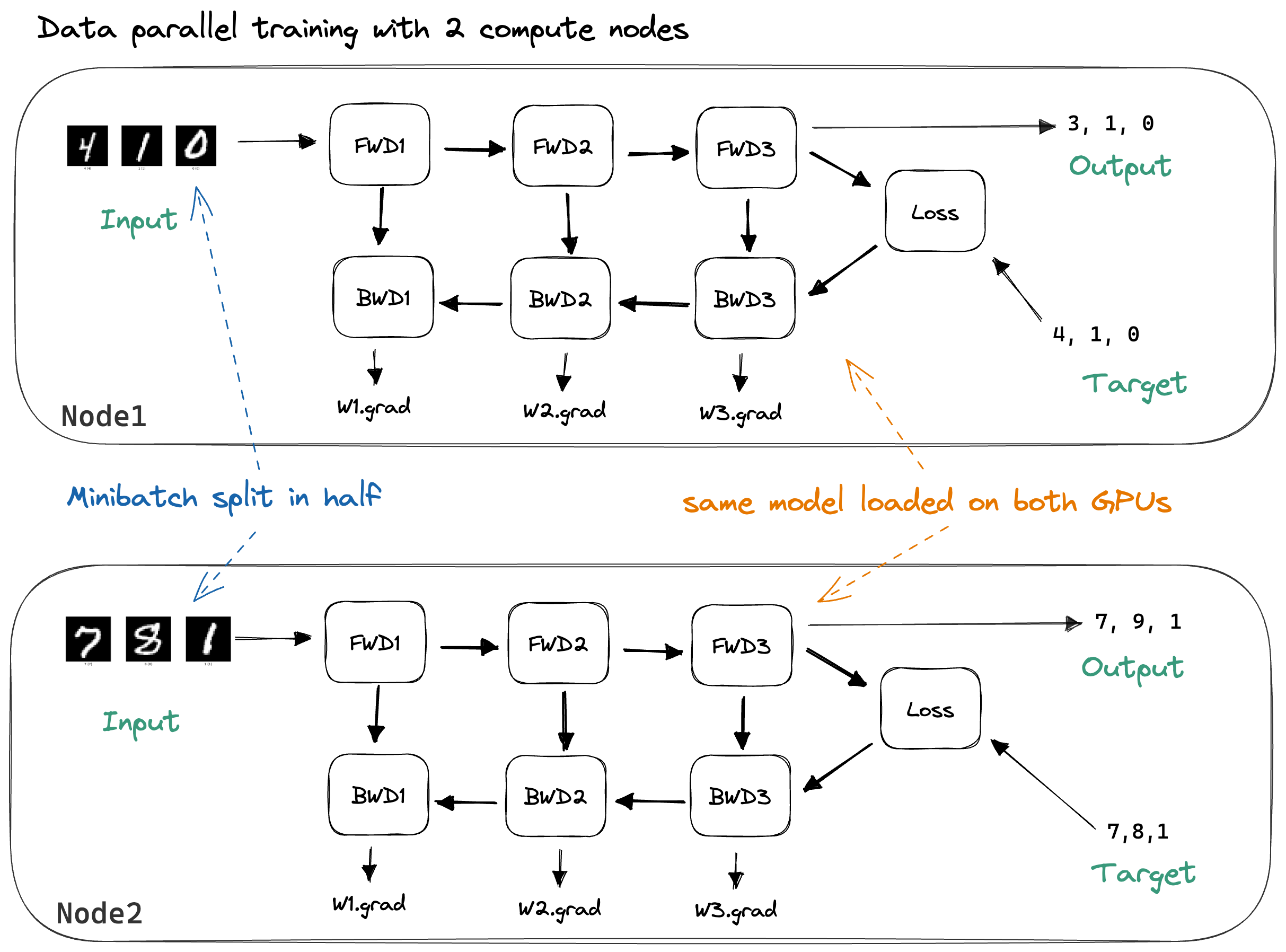
A visual representation of data parallelism. A mini-batch is split, with each half fed into an identical model replica on a separate node. Each node computes its own forward pass, loss, and backward pass to generate local gradients (e.g., W1.grad). These gradients must then be synchronized between the nodes before the weights are updated.

Notice that after the backward pass, each node has gradients computed only on its own data. To perform a gradient descent step that is equivalent to training on the full batch, the nodes need to communicate. This brings us to the communication backbone of distributed training.

The Communication Backbone: Collective Operations

In a distributed system, processes need efficient ways to exchange information. Instead of relying on simple point-to-point sends and receives, distributed training leverages highly optimized collective communication primitives. These operations coordinate data movement across a group of processes simultaneously. For data parallelism, two are fundamental: Broadcast and All-Reduce.

You can think of these as high-level commands orchestrated by a library like PyTorch's torch.distributed, which often uses NVIDIA's NCCL (NVIDIA Collective Communications Library) for blazing-fast performance on GPUs.

Distributed Training with PyTorch: complete tutorial with cloud infrastructure and code

The video "Distributed Training with PyTorch" by Umar Jamil provides exceptionally clear, intuitive explanations of these collective operations using a file-sharing analogy.

Please watch the segment from this section on collective communication. Focus on understanding: Broadcast: How it efficiently distributes data (like initial model weights) from one node to all others using a divide-and-conquer strategy, which is much faster than sending one by one. Reduce: How it aggregates data from all nodes onto a single root node, again using an efficient tree-like structure. All-Reduce: This is the most critical operation for data parallelism. It's logically equivalent to a Reduce (e.g., summing all gradients onto one node) followed by a Broadcast (sending the sum back to all nodes). In practice, it's a single, highly optimized operation that ensures every node ends up with the same aggregated result.

With these primitives, we can now refine our understanding of the training loop:

Initialization: The model is initialized on one process (rank 0), and its weights are sent to all other processes using a Broadcast operation.
Gradient Synchronization: After each backward pass, the locally computed gradients on all processes are averaged using an All-Reduce operation.
Update: Each process independently updates its local model weights using the identical, globally-averaged gradients.

PyTorch DDP: An Efficient Implementation

In PyTorch, data parallelism is implemented via the torch.nn.parallel.DistributedDataParallel (DDP) wrapper. It's the successor to the simpler torch.nn.DataParallel (DP) and is vastly more performant. Your computer science background will appreciate the key difference: DDP uses multiprocessing (one process per GPU), avoiding the Python Global Interpreter Lock (GIL) contention that plagues the multithreaded approach of DP.

DDP also incorporates several key optimizations to minimize the time GPUs spend waiting for communication.

Computation-Communication Overlap: Instead of waiting for the entire backward pass to complete before starting to communicate gradients, DDP begins the all-reduce operation as soon as the gradients for a layer are computed. The communication for earlier layers can thus happen in parallel with the gradient computation for later layers, hiding the communication latency.
Gradient Bucketing: Sending many small gradient tensors over the network is inefficient due to per-operation overhead. DDP groups gradients into larger "buckets" and all-reduces an entire bucket once it's full. This reduces the number of communication calls and improves network bandwidth utilization.

This diagram illustrates gradient bucketing. Gradients for multiple parameters (param0, grad0, param1, grad1) are grouped into a bucket. The all-reduce operation is performed on the entire bucket at once, rather than on each individual gradient tensor, improving communication efficiency.

The following video explains these practical PyTorch optimizations in detail.

Distributed Training with PyTorch: complete tutorial with cloud infrastructure and code

This segment from Umar Jamil's tutorial dives into the clever optimizations within PyTorch's DDP implementation.

Watch the clip from this section. Focus on how the computation-communication overlap works during the backward pass and how bucketing makes this communication more efficient.

Beyond Naive Data Parallelism: ZeRO

So far, our data parallel strategy has one significant drawback: memory redundancy. Every GPU holds a complete replica of:

The model parameters.
The gradients.
The optimizer states (e.g., the momentum and variance buffers for the Adam optimizer, which can be 2x the size of the parameters themselves).

This redundancy means that if a model is too large to fit in one GPU's memory, data parallelism alone cannot help. The solution is an advanced form of data parallelism known as ZeRO (Zero Redundancy Optimizer), which is the algorithm behind PyTorch's Fully Sharded Data Parallelism (FSDP).

ZeRO's core insight is that not all of this information is needed on every GPU at all times. It systematically eliminates this redundancy by "sharding" (partitioning) the model state across the available devices.

Stanford CS336 Language Modeling from Scratch | Spring 2025 | Lecture 7: Parallelism 1

The Stanford lecture offers a superb conceptual walkthrough of the problem of memory redundancy and the progressive stages of the ZeRO solution.

First, re-watch the end of the data parallelism introduction from this clip to understand the initial analysis of compute, communication, and memory scaling. Note the explicit statement: "Memory scaling, I'm not touching this at all. Right? Every GPU needs to replicate the number of parameters... it's pretty bad for memory scaling." Next, watch the segment from this section which details the memory consumption. The diagram showing that optimizer states dominate parameter-related memory is a crucial insight. Now, watch the explanation of ZeRO Stage 1 from here. This is the most important conceptual leap. It answers the question: "How can we shard the optimizer state?" The key is a reduce-scatter operation to give each GPU the gradients for the parameter shard it's responsible for, followed by an all-gather to reconstruct the full, updated parameters. The magic is that the total communication volume remains the same as a standard all-reduce. Finally, get a high-level overview of ZeRO Stage 3 (FSDP) from this clip. Here, everything is sharded, including the parameters. The parameters for a given layer are materialized on-demand via an all-gather just before they are needed, and then discarded. This provides massive memory savings at the cost of increased communication, which is made efficient by overlapping it with computation.

ZeRO-FSDP represents the state of the art for data parallelism. It allows for training models of enormous size by ensuring that the memory required per GPU for parameters, gradients, and optimizer states scales inversely with the number of GPUs.

Conclusion

In this lesson, we have moved from single-device training to the world of distributed systems, focusing on the foundational strategy of data parallelism. This approach allows us to dramatically accelerate training by leveraging the combined computational power of multiple devices.

Key Takeaways:

Data Parallelism works by replicating a model across multiple devices and feeding each replica a different slice of the data batch.
It primarily addresses the compute bottleneck, enabling faster training on large datasets.
Synchronization is achieved through collective communication operations, with All-Reduce being the workhorse for averaging gradients.
Modern implementations like PyTorch DDP use optimizations like computation-communication overlap and gradient bucketing to hide latency.
Naive data parallelism is memory-redundant, as every device stores a full copy of the weights, gradients, and optimizer states.
ZeRO / FSDP (Fully Sharded Data Parallelism) solves this by sharding the training state across devices, drastically reducing per-GPU memory usage and enabling the training of much larger models.

Data parallelism is a powerful tool, but it has its limits. It cannot train a model whose individual layers are too large to fit in a single GPU's memory. For that, we need different strategies. In our next lessons, we will explore pipeline parallelism and tensor parallelism, which partition the model itself across devices, completing our toolkit for training truly massive language models.