Welcome to our next lesson on large-scale training techniques. In our previous session, we explored data parallelism, a powerful strategy for accelerating training by replicating a model and splitting the data across multiple devices. We saw how this approach, especially with optimizations like ZeRO/FSDP, tackles the compute bottleneck and reduces memory redundancy. However, we concluded by noting its fundamental limitation: what happens when the model itself is simply too large to fit into the memory of a single GPU?
This lesson directly addresses that challenge by introducing model parallelism. Instead of replicating the model, we will partition the model's parameters across multiple devices. We will focus specifically on pipeline parallelism, a technique that splits a model vertically, assigning different layers to different devices. Your background in DevOps and distributed systems will provide a strong foundation for understanding the data flow and coordination challenges inherent in this approach.
Our objective is to describe pipeline parallelism and explain how it enables training models that would otherwise be impossibly large for a single device. We'll start with the core concept, analyze its primary inefficiency—the "pipeline bubble"—and then examine the clever solution of micro-batching that makes it practical.
The Core Idea: An Assembly Line for Layers
At its heart, pipeline parallelism is an intuitive concept. Imagine a deep neural network as an assembly line. Instead of one worker (GPU) performing all the steps (layers), we distribute the steps among multiple workers. Each worker is responsible for a specific sequence of layers.
If we have a model with layers and a cluster of GPUs, we can partition the model into stages.
- GPU 0 (Stage 0) holds layers 1 to .
- GPU 1 (Stage 1) holds layers to .
- ...and so on, until GPU holds the final set of layers.
The training process then proceeds as a forward and backward pass through this distributed assembly line.
Training extremely large neural networks across thousands of ...
This article by Jeremy Jordan provides an excellent and clear explanation of the pipeline parallelism workflow.
Please read the section on Pipeline parallelism, starting from the initial explanation. Pay close attention to the description of how the forward pass passes activations between GPUs and how the backward pass propagates gradients in reverse.
As you've just read, the process is sequential. During the forward pass, a batch of data is processed by GPU 0. Its output—the activation from the last layer on that device—is then sent across the network to GPU 1, which uses it as input. This continues until the final stage, GPU , computes the model's output and the loss. The backward pass works in reverse: GPU computes gradients and passes the gradient of its input activations back to GPU , and so on, until GPU 0 computes the gradients for the first set of layers.
The Problem: The Pipeline Bubble
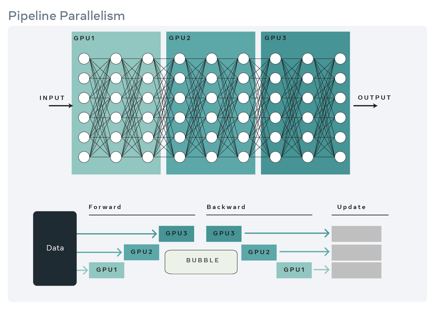
This naive, sequential processing introduces a significant performance issue. While one GPU is working, all other GPUs in the pipeline are idle, waiting for their turn. This period of inactivity is known as the pipeline bubble, and it represents a massive waste of computational resources.

In naive pipeline parallelism, a batch is processed sequentially across devices. The white space, labeled "Bubble," represents idle machine time where GPUs are waiting, leading to poor utilization.
To understand this inefficiency more concretely, let's trace the flow of a single batch.
Ultimate Guide To Scaling ML Models - Megatron-LM | ZeRO | DeepSpeed | Mixed Precision
The video "Ultimate Guide To Scaling ML Models" by Aleksa Gordić offers a great visual walkthrough of setting up a pipeline and the resulting bubble.
First, watch the segment from the beginning to see how a Transformer model is conceptually split across four devices. Then, continue from the next section, which demonstrates step-by-step why this naive approach leads to most devices being idle during both the forward and backward passes.
The "bubble" is the Achilles' heel of simple pipeline parallelism. If we have GPUs, each GPU is active for only of the time for a single batch pass. Our goal is to maximize parallel execution, but this approach serially chains the work, defeating the purpose.
The Solution: Micro-batching
The solution to the pipeline bubble is to break a large data batch into many smaller micro-batches. This allows the pipeline stages to process different micro-batches concurrently in a staggered fashion, much like a real-world assembly line.
Here’s how it works:
- GPU 0 processes the first micro-batch and sends its output activations to GPU 1.
- As GPU 1 starts working on the first micro-batch, GPU 0 immediately begins processing the second micro-batch.
- As GPU 2 starts on the first micro-batch, GPU 1 works on the second, and GPU 0 starts on the third.
This interleaving of computation significantly reduces idle time. While there is still a "ramp-up" phase at the beginning and a "ramp-down" phase at the end where the pipeline is not full, the majority of the time is spent with all GPUs working in parallel.
This diagram contrasts naive pipeline parallelism (top) with micro-batching (bottom). By splitting the data into smaller chunks, computation can be interleaved across GPUs, shrinking the "bubble" of idle time and dramatically increasing overall device utilization.
The following video segment explains this crucial optimization.
Ultimate Guide To Scaling ML Models - Megatron-LM | ZeRO | DeepSpeed | Mixed Precision
This part of Aleksa Gordić's video clearly illustrates how micro-batching fills the pipeline.
Please watch from this segment. Notice how the number of active devices increases over time until the pipeline is full. The video also mentions an important empirical rule from the GPipe paper: to achieve near-linear scaling, the number of micro-batches m should be significantly larger than the number of pipeline stages K, often m \ge 4K.
Each device accumulates the gradients for all micro-batches locally. Once the entire batch has been processed, a single synchronized weight update is performed. This ensures that the final model update is mathematically equivalent to having processed the large global batch on a single, giant device.
A Look Under the Hood: Implementation in Code
Understanding the concept is one thing; seeing how it's implemented provides a deeper appreciation for the engineering involved. Modern frameworks like Megatron-DeepSpeed (which powers models like BLOOM) provide robust implementations of these parallelism strategies. From your DevOps perspective, you can think of each GPU as a worker process with a specific rank, and the parallelism logic is determined by this rank's position in the device topology.
The following video provides a code-level walkthrough of how pipeline parallelism is implemented in the BLOOM codebase. It shows exactly how the model's layers are assigned to different devices and how data is communicated between them.
BigScience BLOOM | 3D Parallelism Explained | Large Language Models | ML Coding Series
In "BigScience BLOOM | 3D Parallelism Explained," Aleksa Gordić steps through the Megatron-DeepSpeed code, revealing the practical implementation of pipeline parallelism.
This is a more in-depth resource. Focus on these key parts: Topology Setup: Watch from this section to understand the concept of a device topology, where GPUs are organized into pipeline stages and model parallel groups. Layer Allocation: See how layers are assigned to devices from this clip. The code calculates num_layers per stage and uses a rank-based offset to build the correct slice of the model on each device. Forward Pass Logic: From this segment, observe the receive_forward function. Notice the conditional logic: if a device is in the first stage, it gets data from the data loader; otherwise, it waits to receive activations from the previous stage. Full Pipeline Flow: The final recap from this part puts it all together. It traces how the first stage handles embeddings, intermediate stages pass activations, and the last stage calculates the final loss. This is the complete picture of the "assembly line" in action.
This code-level view demystifies the process, showing that pipeline parallelism is a result of careful, rank-aware conditional logic that controls which layers are instantiated and how data is passed between processes.
Conclusion
Today, we've added a crucial tool to our large-scale training toolkit. Where data parallelism falls short—when the model itself is too large for a single device—pipeline parallelism provides a direct solution by partitioning the model's layers across a chain of devices.
Here are the key takeaways:
- Pipeline Parallelism splits a model inter-layer, assigning consecutive blocks of layers to different devices, forming a "pipeline."
- It directly solves the problem of a model's memory footprint exceeding that of a single GPU.
- The naive implementation is highly inefficient due to the pipeline bubble, where only one device is active at a time.
- Micro-batching is the standard solution, enabling staggered, concurrent execution across devices to dramatically improve utilization.
- The implementation involves distinct logic for the first, intermediate, and last stages of the pipeline to manage data input, activation passing, and loss computation.
Pipeline parallelism is a foundational technique, but it's often not the whole story. What if a single Transformer layer, with its massive weight matrices, is itself too large for one GPU? Splitting the model between layers won't help. For that, we need a way to split the computation within a layer. This is the domain of our next topic: tensor parallelism.