Tensor Parallelism: Scaling Large Model Layers

From Inter-Layer to Intra-Layer Parallelism

First, let's firmly distinguish between the two types of model parallelism we've discussed. Pipeline parallelism performs an inter-layer split, where different GPUs are responsible for different, sequential chunks of the model. Tensor parallelism performs an intra-layer split, where multiple GPUs collaborate to execute a single, large operation, like a matrix multiplication.

This intra-layer approach was famously detailed in the Megatron-LM paper, and as such, is often called "Megatron-style" tensor parallelism. Let's dive into how it works.

Parallelizing the MLP Block: A Tale of Two GEMMs

The MLP block in a standard Transformer consists of two linear layers (which are primarily General Matrix Multiplies, or GEMMs) with a non-linear activation function, like GeLU, in between. We can represent this as:

1. $Y=\text{GeLU}(XA)$
2. $Z=YB$

Here, $X$ is the input activation tensor, and $A$ and $B$ are the large weight matrices. Our goal is to split the computations involving $A$ and $B$ across multiple GPUs.

Let's consider a simple case of splitting across two GPUs. The key challenge lies in choosing a splitting strategy that preserves the mathematical correctness of the operation while minimizing communication between the GPUs.

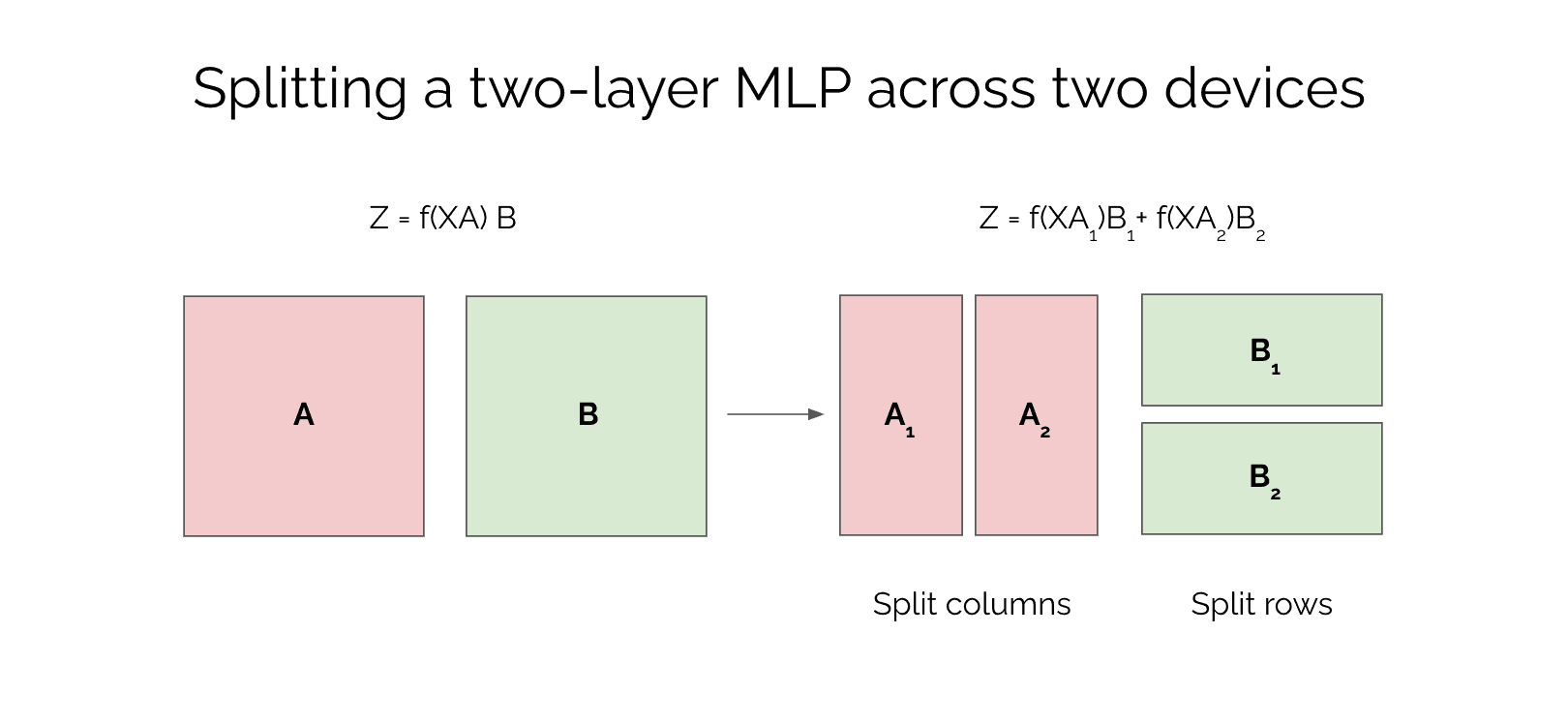
A high-level view of splitting a two-layer MLP. The first weight matrix A is split by columns, while the second matrix B is split by rows. This specific pattern is crucial for efficiency.

The article "An illustrated deep-dive into Megatron-style tensor parallelism" provides an exceptional step-by-step derivation of this process. It's one of the clearest explanations available.

As you've just read, the choice of how to split the first matrix, $A$, is dictated by the non-linear activation function.

• Row-wise split (the "bad" option): If we split $A$ by rows, so $A=\left[\begin{array}{c}{A}_1\\ A_2\end{array}\right]$, the computation becomes $Y=\text{GeLU}(X_1{A}_1+X_2{A}_2)$. Because the GeLU function is non-linear, we have $\text{GeLU}(a+b)\ne \text{GeLU}(a)+\text{GeLU}(b)$. This means we would be forced to sum the partial products $X_1{A}_1$ and $X_2{A}_2$ before applying GeLU. This summation is a communication-heavy all-reduce operation, and needing it so early negates much of the benefit of parallelism.
• Column-wise split (the "good" option): By splitting $A$ by columns, so $A=[A_1,A_2]$, the computation becomes $[Y_1,Y_2]=[\text{GeLU}(X{A}_1),\text{GeLU}(X{A}_2)]$. Here, each GPU can compute its part of the operation and apply GeLU independently, with no communication required. This is the key insight of Megatron-style parallelism.

Now, the output of this first step, $Y=[Y_1,Y_2]$, is a sharded tensor. This sharded tensor becomes the input to the second linear layer, $Z=YB$. To make the matrix multiplication dimensions compatible, we must now split the second weight matrix, $B$, row-wise: $B=\left[\begin{array}{c}{B}_1\\ B_2\end{array}\right]$.

The full computation on the two GPUs is:

• GPU 1 computes $Z_1=Y_1{B}_1$
• GPU 2 computes $Z_2=Y_2{B}_2$

The final result should be $Z=Z_1+Z_2$. At this stage, communication is unavoidable. The partial results $Z_1$ and $Z_2$ must be summed together across the devices using an all-reduce operation.

The brilliant stroke of this design is that it requires only one synchronization point (the final all-reduce) in the forward pass of the entire two-layer MLP block.

The following diagram from the original Megatron-LM paper illustrates this flow. The operator $g$ represents a forward-pass all-reduce, while $f$ represents its conjugate for the backward pass (an all-reduce of gradients).

This figure from the Megatron-LM paper shows the data flow for both (a) MLP and (b) Self-Attention blocks under tensor parallelism. Notice the column-wise split for the first matrix (XA) and row-wise for the second (YB), with a single synchronization (g) at the end of the block.

To see this logic animated, let's turn back to Aleksa Gordić's video.

Parallelizing the Self-Attention Block

The same principle can be applied to the self-attention block. In fact, it's even more natural here because the multi-head attention mechanism is already composed of independent computations—one for each head.

The core idea is to split the attention heads across the available GPUs.

1. The large projection matrices for Query, Key, and Value ($W^Q,W^K,W^V$) are split column-wise across the num_heads dimension.
2. Each GPU now holds the weights for a subset of the attention heads. It can independently compute the Q, K, and V vectors for its heads, perform the scaled dot-product attention, and produce an output for its subset of heads. All of this happens with zero communication.
3. The final output projection layer, which combines the results from all heads, has its weight matrix ($W^O$) split row-wise.
4. Each GPU computes a partial result by multiplying its attention head outputs with its shard of the $W^O$ matrix.
5. Finally, just as with the MLP block, an all-reduce operation sums these partial results to produce the final output of the attention block.

This elegant parallelization results in just one all-reduce in the forward pass and one in the backward pass for the entire multi-head attention block.

The Cost of Communication: System-Level Tradeoffs

We have established a powerful technique, but it doesn't come for free. Tensor parallelism introduces high-frequency communication. Unlike data parallelism, which requires one all-reduce per batch, or pipeline parallelism, which involves passing activations between stages, tensor parallelism requires all-reduce operations inside every Transformer layer.

This has profound implications for hardware and system architecture, a topic where your DevOps expertise provides a unique lens. These all-reduce operations are extremely sensitive to network latency and bandwidth.

• Intra-node communication: Communication between GPUs within the same physical server is often handled by ultra-fast, low-latency interconnects like NVIDIA's NVLink.
• Inter-node communication: Communication between different servers across a network (e.g., via Infiniband or Ethernet) is significantly slower.

Because of this, tensor parallelism is almost exclusively used for GPUs within a single node. The communication overhead would be prohibitively expensive across nodes. This creates a practical limit on the tensor parallel size, typically 8 or 16 GPUs, corresponding to the number of GPUs in a high-density server.

The following video provides an expert perspective on these tradeoffs, backed by empirical data.

This analysis reveals that scaling LLMs is not just about using one technique, but about composing them intelligently. A typical setup for a massive model might use tensor parallelism within each node, pipeline parallelism across nodes, and data parallelism across replicas of the entire pipeline.

Conclusion

Today we've completed our trio of large-scale training strategies by adding tensor parallelism to our toolkit. While data parallelism replicates the model and pipeline parallelism splits it between layers, tensor parallelism gives us the fine-grained ability to split the computations within a single, massive layer.

Here are the key takeaways:

• Tensor Parallelism splits a model's computations intra-layer, partitioning large weight matrices (tensors) and their associated GEMMs across multiple devices.
• It is essential when a single model layer is too large to fit in one GPU's memory.
• The partitioning scheme is carefully designed to minimize communication, typically involving a column-wise split followed by a row-wise split in MLP and attention blocks to delay synchronization.
• This introduces high-frequency all-reduce communication, making it highly sensitive to network performance and best suited for fast intra-node interconnects like NVLink.
• Effective scaling often involves a hybrid approach, combining data, pipeline, and tensor parallelism, each playing to its strengths at different levels of the hardware topology.

With these three parallelism techniques, we now have a comprehensive understanding of the engineering required to train models at the scale of billions or even trillions of parameters. We know the mechanisms for scaling. In our next module, we will explore the principles that guide these scaling efforts: the Scaling Laws that describe the predictable relationships between model performance, size, data, and compute.