Mixed-Precision Training: Balancing Speed and Accuracy

The Promise of Lower Precision

At its heart, a neural network is a massive collection of floating-point numbers—weights, biases, activations, and gradients. By default, these are stored in a 32-bit single-precision format, commonly known as float32 or FP32. Your computer science background gives you an innate understanding that data representation is a series of trade-offs. Let's make that concrete for floating-point numbers.

A floating-point number is typically composed of three parts: a sign bit, an exponent, and a fraction (or mantissa). The number of bits allocated to the exponent determines the range of numbers that can be represented (how large or small they can be), while the bits for the mantissa determine the precision (how many significant digits can be stored).

To see exactly how this works for FP32 and its lower-precision counterparts, the following video provides a superb from-the-ground-up explanation.

The idea behind mixed-precision training is simple: if we can use fewer bits, say 16, we can cut our memory usage in half. This applies to the model's weights, the gradients, and the memory-hungry activations we discussed in the last lesson. There are two main 16-bit formats used in deep learning: float16 (FP16) and bfloat16 (BF16).

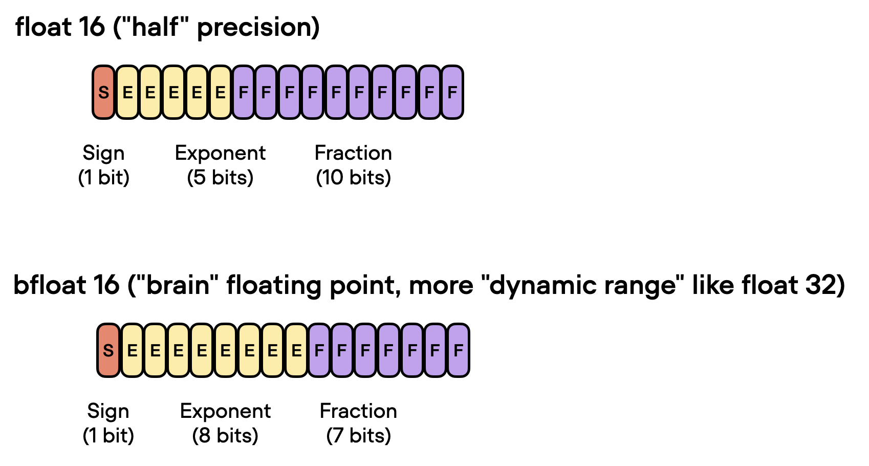
A comparison of the bit allocation in float16 ("half" precision) and bfloat16 ("brain" float). Note the critical difference in exponent and fraction bits.

As the image shows, they make a different trade-off:

• float16 (FP16): Allocates 5 bits for the exponent and 10 for the fraction. Compared to FP32, it has a drastically smaller range but retains reasonable precision.
• bfloat16 (BF16): Allocates 8 bits for the exponent (the same as FP32!) and 7 for the fraction. It has the same massive range as FP32 but much lower precision.

This reduction in bits yields two major benefits:

1. Reduced Memory Footprint: Halving the bits per number roughly halves the memory required for the model, its gradients, and optimizer states. This enables training larger models or using larger batch sizes, synergizing perfectly with gradient accumulation.
2. Increased Computational Speed: Moving fewer bits around reduces memory bandwidth bottlenecks. More importantly, modern GPUs (like NVIDIA's A100 and H100 series) have specialized hardware units called Tensor Cores that execute 16-bit matrix multiplications far faster than 32-bit operations.

The following segment of the video explains these benefits in more detail.

The Peril: Numerical Instability

Given these advantages, an obvious question arises: why not just cast everything to FP16 and enjoy the benefits? The answer lies in its limited range.

Gradient Underflow

The biggest problem is gradient underflow. During training, especially in deep networks, it's common for gradient values to become extremely small. The smallest positive normalized number FP16 can represent is approximately $6\times 10^{-5}$. Any gradient smaller than this gets "flushed to zero." The update for that weight becomes zero, and the model simply stops learning.

This isn't a theoretical concern. The NVIDIA documentation for mixed precision provides a stark visualization of this problem.

The video we've been watching provides a brilliant low-level explanation for why even updates that don't underflow can be lost.

The Solution: The Mixed-Precision Recipe

To safely harness the power of FP16, we can't use it naively. Instead, we use a "mixed" approach, combining FP16 and FP32 in a clever recipe. This recipe has two main ingredients.

1. Maintaining an FP32 Master Copy of Weights

The first problem we saw was that even if a gradient survives, the update weight += learning_rate * gradient might result in a value too small to change the FP16 weight.

The solution is to perform the update in a higher-precision format. We keep a master copy of the model weights in FP32. The training loop then looks like this:

1. For the forward and backward pass, use a temporary FP16 copy of the weights to get the speed and memory benefits.
2. After computing the gradients, use them to update the FP32 master copy. In FP32, the tiny updates can be correctly accumulated over many steps.
3. Copy the updated FP32 weights back to the FP16 format for the next iteration.

2. Loss Scaling

Maintaining an FP32 master copy solves the update problem, but it doesn't solve the initial gradient underflow issue. If the gradients are already zero before they even reach the optimizer, there's nothing to update.

The solution is loss scaling. The logic is as follows:

1. Before the backward pass, multiply the loss (a single scalar) by a large scaling factor, say $S=8192$.
2. By the chain rule of calculus, all the gradients computed during the backward pass will automatically be scaled by this same factor $S$.
3. This scaling pushes the tiny gradient values up into the representable range of FP16, preventing them from becoming zero.
4. Before the optimizer updates the FP32 master weights, the gradients are unscaled by dividing them by $S$. This returns them to their correct magnitude, ensuring the weight update is correct.

This process ensures that gradient information is preserved through the FP16 backpropagation. The final mixed-precision training loop combines both techniques.

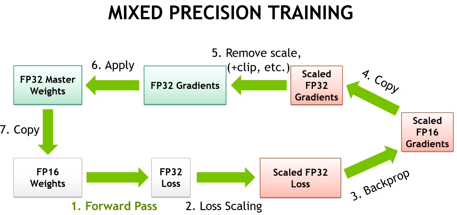
The full mixed-precision training algorithm. This visualizes the interplay between FP16 and FP32 copies of weights and gradients, as well as the loss scaling and unscaling steps.

The video explains this final, crucial piece of the puzzle.

In practice, the scaling factor $S$ is not fixed. Modern frameworks use dynamic loss scaling, where the training process automatically adjusts $S$. It starts with a large $S$, and if it detects an overflow (gradients becoming inf or NaN), it reduces $S$ and skips the update for that step. If training proceeds for many steps without overflow, it attempts to increase $S$ again, always trying to use the maximum dynamic range of FP16 without causing instability.

BFloat16: A Modern, Simpler Alternative

The complexity of FP16 training (master weights, dynamic loss scaling) stems entirely from its limited range. This led to the development of bfloat16 (BF16). By having the same 8-bit exponent as FP32, BF16 has the same dynamic range as FP32.

This means gradient underflow and overflow are no longer significant concerns. BF16 training is therefore much simpler:

• Loss scaling is generally not required.
• You still benefit from FP32 master weights to accumulate small updates with higher precision, but the most complex part of the process is removed.

The trade-off is BF16's lower precision (7 mantissa bits vs. FP16's 10). However, it turns out that deep neural networks are remarkably resilient to this kind of noise, but extremely sensitive to the range issues that plague FP16. For this reason, on modern hardware that supports it (e.g., NVIDIA A100/H100, Google TPUs), BF16 is the preferred format for mixed-precision training.

Conclusion

In this lesson, we have dissected mixed-precision training, a cornerstone of efficient, large-scale model pre-training. We've seen that it's not a simple switch, but a carefully engineered system that balances computational efficiency with numerical reality.

Here are the key takeaways:

• The Goal: Reduce memory usage and increase speed by using 16-bit floating-point formats (FP16, BF16) instead of the standard 32-bit (FP32).
• The Problem with FP16: Its limited dynamic range leads to gradient underflow (small gradients becoming zero) and lost weight updates, which stalls training.
• The FP16 Solution (Mixed Precision):
  1. Use FP16 for forward/backward passes to save memory and leverage fast hardware.
  2. Maintain a master copy of weights in FP32 to accurately accumulate small updates.
  3. Use (dynamic) loss scaling to shift small gradients into the representable range of FP16, preventing underflow.
• The Modern Solution (BF16): bfloat16 has the same range as FP32, largely eliminating the underflow/overflow problems. This makes training much simpler as loss scaling is typically unnecessary, making BF16 the preferred format on supporting hardware.

We have now covered the two primary techniques for managing computational resources on a single GPU: gradient accumulation for handling large batches, and mixed-precision training for optimizing memory and speed at the data-type level. With these tools, we can train much larger and more powerful models. However, even these techniques have their limits. To train truly massive models like GPT-3, we must scale beyond a single device. In our next lesson, we will begin exploring how to do this, starting with data parallelism.