Euler Integration: Velocity and Acceleration in Fixed Update

The Physics of Motion

At the heart of physics simulation are the fundamental equations of motion, which you'll recognize from your physics courses. Given an object with mass $m$, and a net force $F$ acting on it, its acceleration $a$ is given by Newton's second law:

$a=\frac{F}{m}$

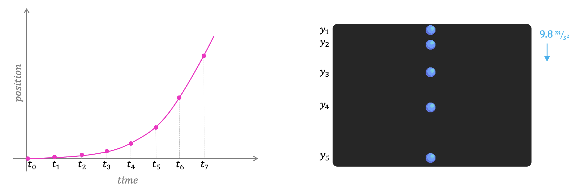
Acceleration is the rate of change of velocity ($v$) over time, and velocity is the rate of change of position ($x$) over time. This gives us a system of first-order ordinary differential equations:

1. $\frac{dv}{dt}=a$
2. $\frac{dx}{dt}=v$

To simulate this on a computer, we can't solve these equations continuously. Instead, we approximate the solution by taking small, discrete steps forward in time. This process is called numerical integration.

Euler Integration: Stepping Through Time

The simplest method for numerical integration is called Euler integration. It works by approximating the next state of a system (position and velocity) using its current state and a small time step, which we'll call delta time or dt.

Let's start with a formal derivation, which will likely feel familiar from your calculus or numerical methods courses.

As the video showed, we can approximate the change in position and velocity over a small time step dt as:

• change in position ≈ velocity * dt
• change in velocity ≈ acceleration * dt

This leads to a straightforward implementation. However, the order in which we calculate these updates matters a great deal.

Key Takeaways from "Integration Basics":

1. Explicit Euler Integration:

   // Update position using the OLD velocity
   position = position + velocity * dt; 
   // Update velocity
   velocity = velocity + acceleration * dt;
   

   This method is simple but often unstable. In many physical systems (like springs), it tends to add energy over time, causing simulations to "explode".

2. Semi-Implicit Euler Integration:

   // Update velocity FIRST
   velocity = velocity + acceleration * dt;
   // Update position using the NEW velocity
   position = position + velocity * dt; 
   

   By simply swapping the order of operations, we get a much more stable integrator. It tends to conserve energy better and is the standard choice for physics in most commercial game engines due to its simplicity and stability. We will use this method.

The Problem with Frame Rate: Why We Need a Fixed Timestep

Now that we know how to step our simulation forward by dt, we need to decide what value dt should have. A naive approach is to measure the time taken by the last frame and use that as dt. This is called a variable timestep, and it's a recipe for disaster in physics simulations.

Let's explore why this is a problem and what the correct solution is.

The video makes it clear: to have a stable, deterministic, and predictable physics simulation, we must separate the physics update rate from the rendering frame rate. The physics simulation should always advance in constant, fixed time steps.

Now, let's dive into the implementation details of this fixed-step loop using a technique called an accumulator.

The core idea is:

1. Measure the real time that has passed since the last frame (frameTime).
2. Add this frameTime to an accumulator variable.
3. Run the physics update in a while loop, with a fixed dt, as long as the accumulator has enough time stored in it.
4. Subtract dt from the accumulator for each physics step taken.
5. Render the game state once per frame, after the physics loop is done.

Implementation: Building the Physics System

Let's integrate these concepts into our C engine.

1. The PhysicsBody Component

First, we need a component to store the physical properties of an entity. In your components.h (or a new physics_component.h), define the PhysicsBody struct.

// In your components header file

// ... other component structs

typedef struct {
    vec3 velocity;
    vec3 acceleration;
    float mass;
} PhysicsBody;

// Remember to add it to your World struct and entity manager functions!

You'll need to update your entity/world management code to handle this new component, just as you did for Transform and Collider. For now, we'll only use velocity and acceleration. We'll use mass in the next lesson.

2. The physics_system

Create a new pair of files: physics_system.h and physics_system.c.

physics_system.h

#ifndef PHYSICS_SYSTEM_H
#define PHYSICS_SYSTEM_H




#include "ecs.h" // Your entity-component-system header

// Updates the position of all entities with a physics body
// using semi-implicit Euler integration.
void physics_system_update(World* world, float dt);




#endif // PHYSICS_SYSTEM_H

physics_system.c

#include "physics_system.h"
#include <cglm/cglm.h> // Or your math library

void physics_system_update(World* world, float dt) {
    // Iterate over all entities that have both a Transform and a PhysicsBody
    for (int i = 0; i < world->entity_count; ++i) {
        // Check if entity has the required components
        if ((world->entity_masks[i] & (COMPONENT_TRANSFORM | COMPONENT_PHYSICS_BODY)) 
            == (COMPONENT_TRANSFORM | COMPONENT_PHYSICS_BODY)) {
            
            Transform* transform = &world->transforms[i];
            PhysicsBody* physics = &world->physics_bodies[i];

            // --- Semi-implicit Euler Integration ---

            // 1. Update velocity
            vec3 scaled_accel;
            glm_vec3_scale(physics->acceleration, dt, scaled_accel);
            glm_vec3_add(physics->velocity, scaled_accel, physics->velocity);

            // 2. Update position
            vec3 scaled_vel;
            glm_vec3_scale(physics->velocity, dt, scaled_vel);
            glm_vec3_add(transform->position, scaled_vel, transform->position);
        }
    }
}

(Note: You might need to adjust the code to match your specific ECS implementation, such as how you access components.)

3. The New Main Loop in main.c

Finally, let's restructure your main loop in main.c to use the fixed timestep with an accumulator.

// In main.c



#include "physics_system.h"
// ... other includes

// You will also need a function to get high-resolution time.
// On Windows, you can use QueryPerformanceCounter.
// On Linux/macOS, you can use clock_gettime.
// For now, let's assume you have a function `get_time_in_seconds()`.
// GLFW provides one: glfwGetTime().

int main(void) {
    // ... Initialization code (window, ECS, entities etc.) ...

    // --- Create a test entity ---
    int cube_entity = world_create_entity(&world);
    entity_add_transform(&world, cube_entity, (Transform){{0.0f, 0.0f, -5.0f}});
    entity_add_physics_body(&world, cube_entity, (PhysicsBody){
        .velocity = {1.0f, 1.0f, 0.0f},      // Give it some initial velocity
        .acceleration = {0.0f, -0.5f, 0.0f}, // Give it some downward acceleration
        .mass = 1.0f
    });
    // Add a mesh/model component so you can see it!

    // --- Fixed Timestep Game Loop ---
    double t = 0.0;
    const double dt = 1.0 / 60.0; // Physics timestep (e.g., 60 Hz)

    double currentTime = glfwGetTime();
    double accumulator = 0.0;

    while (!glfwWindowShouldClose(window)) {
        double newTime = glfwGetTime();
        double frameTime = newTime - currentTime;
        currentTime = newTime;

        accumulator += frameTime;

        while (accumulator >= dt) {
            // Update physics with a fixed delta time
            physics_system_update(&world, (float)dt);
            
            accumulator -= dt;
            t += dt;
        }

        // --- Rendering ---
        // Your existing rendering code goes here.
        // It runs once per frame, independent of physics updates.
        glClear(GL_COLOR_BUFFER_BIT | GL_DEPTH_BUFFER_BIT);
        
        // render_system_draw_entities(&world, ...);

        glfwSwapBuffers(window);
        glfwPollEvents();
    }

    // ... Cleanup ...
    return 0;
}

When you run this code, you should see your cube move diagonally up and to the right, while slowly accelerating downwards, tracing a parabolic arc. This movement will be smooth and consistent, regardless of your computer's speed or the rendering frame rate.

Conclusion

Congratulations! You have just implemented two of the most fundamental concepts in game physics. Your engine now has a proper pulse, with a physics heart beating at a steady, fixed rate.

Key Takeaways:

• Physics simulation is an approximation of continuous motion, solved with numerical integration.
• Semi-implicit Euler is a stable, simple, and effective integration method for games. It's crucial to update velocity before updating position.
• A fixed timestep loop with an accumulator is essential for creating a stable and deterministic physics simulation that is independent of the rendering frame rate.

Preview of the Next Lesson:
Our physics simulation is running, but it's not very dynamic. The acceleration is hard-coded. To make our world interactive, we need to be able to change acceleration on the fly. In the next lesson, you will learn how to apply forces, like gravity, to entities. This will involve using the mass property of the PhysicsBody and the formula a = F/m to calculate acceleration each frame, paving the way for jumping, gravity, and other dynamic behaviors.