Extracting Diffusion Coefficients from RDE Data using the Levich Equation

Welcome back. In our last lesson, we introduced the rotating disk electrode (RDE) as a powerful tool for controlling mass transport. We established that for a mass-transport-limited reaction, the resulting limiting current, $i_{L}$ , is directly proportional to the square root of the electrode's rotation rate, $ω^{1/2}$ . This relationship is captured by the Levich equation.

Today, we will move from the theoretical principle to practical application. Your goal for this lesson is to learn how to interpret experimental RDE data using the Levich equation to extract a fundamental physical property of a redox species: its diffusion coefficient (D). As someone developing and testing new catalyst materials, being able to determine such parameters is a key skill that separates routine testing from rigorous quantitative analysis, allowing you to build a more complete picture of your electrochemical system.

From Voltammograms to the Levich Plot

The first step in this analysis is to perform a "Levich study." As you know from your lab work, this involves recording linear sweep voltammograms (LSVs) at several different rotation rates while keeping all other conditions (like reactant concentration and temperature) constant.

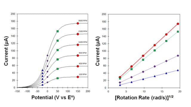
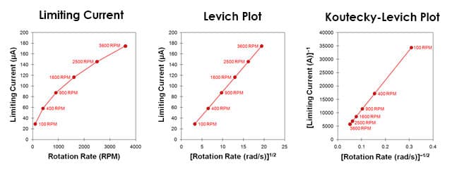
Left: A typical set of LSVs for a redox reaction at increasing rotation rates. Note how the limiting current plateau rises with speed. Right: The limiting current from each curve is plotted against the square root of the rotation rate, forming a Levich plot.

The data you need are the limiting current values, $i_{L}$ , from the plateau region of each voltammogram. By plotting these values against the square root of the corresponding rotation rate ( $ω^{1/2}$ ), you construct a Levich plot.

As predicted by the Levich equation, for a simple, reversible reaction that is purely limited by mass transport, this plot should yield a straight line that passes through the origin. The image below shows the typical data transformation process: from a plot of limiting current versus RPM (non-linear) to the linearized Levich plot.

This figure illustrates the process of creating a Levich Plot (center) from the raw limiting current data (left). The Koutecky-Levich plot (right), which we discussed in the last lesson, is another way to represent the same data.

Calculating the Diffusion Coefficient from the Levich Slope

The power of the Levich plot lies in its slope. Let's recall the Levich equation:

i_{L} = 0.620 n F A D^{2/3} ν^{- 1/6} C^{*} ω^{1/2}

This equation is in the form of a straight line, $y = m x$ , where:

$y = i_{L}$ (the limiting current)
$x = ω^{1/2}$ (the square root of the angular rotation rate)
$m$ is the Levich slope

Therefore, the slope of your Levich plot is equal to all the constant terms in the equation:

slope = 0.620 n F A D^{2/3} ν^{- 1/6} C^{*}

By determining the slope from your experimental data, you can then rearrange the equation to solve for the diffusion coefficient, $D$ .

Levich analysis: the principles - BioLogic Learning Center

This article from BioLogic's learning center clearly outlines how the Levich slope is used to determine the diffusion coefficient.

Please read the section that describes how to construct the Levich plot and use its slope. Pay close attention to the equation provided for the Levich slope, p_{Lc}.

As you just read, with the experimentally determined slope, you can isolate $D^{2/3}$ and then solve for $D$ . The rearranged equation is:

D = (\frac{slope}{0.620 n F A ν ^{- 1/6} C ^{*}})^{3/2}

To perform this calculation, you need the values for all the other parameters:

$n$ : The number of electrons transferred in the reaction.
$F$ : The Faraday constant ( $96, 485 C/mol$ ).
$A$ : The geometric area of the electrode disk.
$ν$ : The kinematic viscosity of the electrolyte solution (a value you would typically look up in literature for your specific electrolyte and temperature).
$C^{*}$ : The bulk concentration of the electroactive species.

A Practical Guide: From Data to Diffusion Coefficient

The following video provides an excellent step-by-step guide on how to perform this analysis, from the raw data to the final calculation. It also highlights the most common and critical sources of error, particularly unit conversions. Your background in chemical engineering makes you appreciate the importance of dimensional analysis, and in electrochemistry, this is paramount.

How to measure the diffusion coefficient using a rotating disk electrode

This video from Pine Research Instrumentation walks through a complete example of calculating a diffusion coefficient from RDE data.

First, watch the section that breaks down each parameter in the Levich equation. Next, pay very close attention to the discussion on common unit conversions. This is arguably the most critical part of the video for avoiding errors in your own work. Finally, watch the full demonstration of the data analysis process, where raw data is plotted, a slope is extracted, and the diffusion coefficient is calculated and compared to a literature value.

As the video emphasized, ensuring all your parameters are in the correct base units is essential for an accurate result. Here is a summary of the key conversions:

Parameter	Symbol	Common Unit	Required Unit for Levich Eq.	Conversion Factor
Limiting Current	$i_{L}$	$μ A$ or $m A$	Amperes (A)	$1 0^{- 6}$ or $1 0^{- 3}$
Rotation Rate	$f$	RPM	rad/s ( $ω$ )	$ω = f \times \frac{2 π}{60}$
Concentration	$C^{*}$	mol/L (M)	mol/cm³	$C_{mol/cm³}^{} = C_{M}^{} \times \frac{1}{1000}$
Electrode Area	$A$	mm²	cm²	$A_{cm²} = A_{mm²} \times \frac{1}{100}$
Kinematic Viscosity	$ν$	cSt	cm²/s	$1 cSt = 0.01 cm²/s$

A Note on Koutecký-Levich Analysis

In the last lesson, we introduced the Koutecký-Levich plot ( $1/ i$ vs. $1/ ω^{1/2}$ ) as a tool to separate kinetic current from mass-transport effects. It's worth noting that the slope of a Koutecký-Levich plot also contains the diffusion coefficient. The Koutecký-Levich equation is:

\frac{1}{i} = \frac{1}{i _{k}} + \frac{1}{B ω ^{1/2}} where B = 0.620 n F A D^{2/3} ν^{- 1/6} C^{*}

The slope of this plot is $1/ B$ . Therefore, you can also determine $D$ from the slope of a Koutecký-Levich plot. This is particularly useful in systems with mixed kinetic and mass-transport control, where a simple Levich plot of the limiting current might not be sufficient. The slope of the K-L plot always reflects the mass transport properties, while the intercept reflects the kinetics.

Conclusion

In this lesson, we bridged the gap between electrochemical theory and experimental practice. You now have a quantitative method to analyze your RDE data to determine a key physical constant.

Key Takeaways:

A Levich plot is a graph of the limiting current ( $i_{L}$ ) versus the square root of the angular rotation rate ( $ω^{1/2}$ ).
For a mass-transport-controlled reaction, this plot is linear, and its slope is defined by the Levich equation.
By measuring the slope and knowing the other experimental parameters ( $n, A, ν, C^{*}$ ), you can calculate the diffusion coefficient (D) of the reactant.
Meticulous attention to unit consistency is absolutely critical for obtaining an accurate result.

Preview of the Next Module:

We have now completed our exploration of the fundamental principles of thermodynamics, the electrode interface, kinetics, and mass transport. You are now equipped with the core theoretical framework needed to understand electrochemical measurements. In the next module, we will begin applying this framework to the workhorses of electrocatalysis research: Cyclic Voltammetry (CV) and Linear Sweep Voltammetry (LSV). We will see how the concepts of potential, kinetics, and mass transport all manifest in the shapes of voltammograms and learn how to extract critical information about your catalysts from them.

Recommended resources

From Voltammograms to the Levich Plot

Calculating the Diffusion Coefficient from the Levich Slope

A Practical Guide: From Data to Diffusion Coefficient

A Note on Koutecký-Levich Analysis

Conclusion