Cyclic Voltammetry: Principles and Waveforms

The Potential Waveform: A Triangular Stimulus

At its core, cyclic voltammetry is an experiment where we apply a specific time-varying potential to a working electrode and measure the resulting current. The "cyclic" part of the name refers to the shape of this potential program: a triangular waveform.

The experiment is controlled by a potentiostat, which linearly sweeps the potential of the working electrode (relative to a reference electrode) with time. A typical CV experiment consists of:

1. Starting at an initial potential ($E_i$).
2. Sweeping the potential at a constant scan rate ($\nu$) to a switching potential ($E_s$). This is the first segment, or forward scan.
3. Reversing the sweep direction and scanning back towards a final potential ($E_f$), which is often the same as the initial potential. This is the second segment, or reverse scan.

Together, the forward and reverse scans make up one cycle. This process can be repeated for multiple cycles. The scan rate, measured in volts per second (V/s) or millivolts per second (mV/s), is a critical experimental parameter that you control.

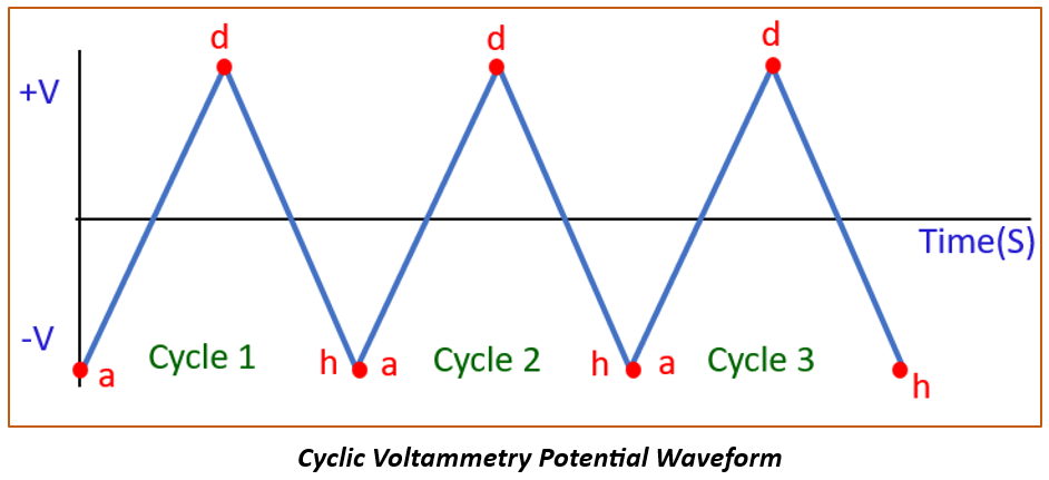
To visualize this potential program and its key parameters, the following video provides a concise overview.

The System's Response: Measuring the Current

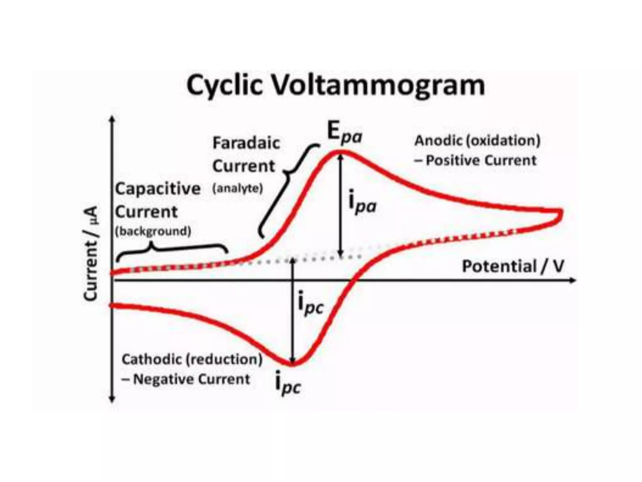
As we apply this triangular potential waveform, we measure the current that flows through the working electrode. A plot of this current (y-axis) versus the applied potential (x-axis) gives us the characteristic cyclic voltammogram.

The total current measured has two main components. Understanding this distinction is fundamental to interpreting a voltammogram correctly.

1. Non-Faradaic Current (Capacitive Current): As you'll recall from our module on the electrode-electrolyte interface, an electrical double layer (EDL) forms at the surface of the electrode. This layer of ions and oriented solvent molecules acts like a capacitor. As we sweep the potential, current must flow to charge or discharge this capacitor. This is the non-Faradaic current because no electron transfer (i.e., no redox chemistry) is occurring. It is often called the background or capacitive current.

2. Faradaic Current: This is the current generated by electron transfer reactions at the electrode surface, named after Michael Faraday. When the applied potential becomes sufficient to either oxidize or reduce a species in the solution, electrons are transferred between the analyte and the electrode, resulting in Faradaic current. This is the component that gives us information about the redox properties of our system and is typically what we are most interested in when studying catalysts.

The video you just watched also provides a clear explanation of how these two types of current arise at the electrode surface.

The Working Principle: From Waveform to Voltammogram

Now, let's connect the applied potential waveform to the measured current to understand why a cyclic voltammogram for a simple, reversible redox process has its iconic "duck" shape. The process relies on the interplay between the potential-dependent reaction kinetics (governed by equations like Butler-Volmer) and mass transport limitations (governed by Fick's laws of diffusion).

To make this concrete, let's walk through a scan. Imagine we have a solution containing only the reduced form (Red) of a reversible redox couple, Red $\rightleftharpoons$ Ox + e⁻.

1. The Three-Electrode System: The experiment uses a three-electrode setup. The potential is controlled between the Working Electrode (WE), where our reaction of interest occurs, and the Reference Electrode (RE), which provides a stable potential. The Counter Electrode (CE) (or auxiliary electrode) passes whatever current is necessary to balance the current at the WE, ensuring the WE-RE potential is maintained accurately without passing significant current through the delicate RE.

2. The Forward (Anodic) Scan: We start at a potential where 'Red' is stable and sweep towards more positive (oxidizing) potentials.

   • Baseline: Initially, the potential is not sufficient to oxidize 'Red'. Only a small capacitive current flows.
   • Onset: As the potential nears the formal potential of the couple ($E^{0^{\prime }}$), oxidation begins. 'Red' at the electrode surface loses electrons, becoming 'Ox', and a Faradaic current begins to flow.
   • Rising Current: The current increases exponentially as the overpotential increases, a region dominated by kinetics.
   • The Peak: As the reaction proceeds, 'Red' near the electrode surface is consumed. To continue reacting, more 'Red' must diffuse from the bulk solution. At the peak of the wave ($i_{pa}$), the rate of reaction becomes limited by the rate of diffusion.
   • Decay: Past the peak, the depletion region for 'Red' expands further into the solution. The diffusion path length increases, so the flux of 'Red' to the surface decreases, causing the current to decay even as the potential becomes more oxidizing.

3. The Reverse (Cathodic) Scan: After reaching the switching potential, the scan is reversed.

   • A high concentration of 'Ox' has now been generated near the electrode surface.
   • As the potential sweeps to more negative values, it becomes favorable to reduce 'Ox' back to 'Red' (Ox + e⁻ $\to$ Red).
   • A similar process occurs in reverse: a cathodic current begins to flow, increases as the potential becomes more reducing, reaches a peak ($i_{pc}$) when the reaction becomes diffusion-limited (this time by the diffusion of 'Ox' to the electrode), and then decays.

This entire sequence creates the characteristic shape. The following article from the Journal of Chemical Education provides a detailed, step-by-step walkthrough of this process, which will solidify your understanding.

Finally, a quick but important practical note. When you look at CVs in different papers or textbooks, you may notice they are sometimes flipped. This is due to two different plotting conventions.

• IUPAC Convention: Anodic (oxidation) current is plotted as positive (up), and cathodic (reduction) current is plotted as negative (down). The potential axis usually goes from negative to positive (left to right). This is the modern standard.
• "Classical" or US Convention: Anodic current is plotted as negative (down), and cathodic current is positive (up). The potential axis often runs from positive to negative.

It's crucial to check the axes and be aware of which convention is being used to interpret the data correctly.

Conclusion

In this lesson, we have established the fundamental principles of cyclic voltammetry. While you've performed this experiment many times, you now have a more formal framework for understanding what is happening at each stage.

Key Takeaways:

• Cyclic voltammetry applies a triangular potential waveform to a working electrode and measures the resulting current. The scan rate is a key experimental parameter that defines the speed of the potential sweep.
• The total measured current is the sum of Faradaic current (from redox reactions) and non-Faradaic current (from charging the electrical double layer).
• The characteristic peak shape of a voltammogram arises from a transition between kinetic control (at the foot of the wave) and mass transport (diffusion) control (at and beyond the peak).
• The forward scan probes one direction of the redox reaction (e.g., oxidation), while the reverse scan probes the other (e.g., reduction), providing a complete "cycle" of information.

Preview of the Next Lesson:

Now that we understand the origin of the voltammogram's shape, we can begin to extract quantitative information from it. In our next lesson, we will focus on identifying and interpreting the anodic and cathodic peaks. We will learn how their position and magnitude relate to the thermodynamics and kinetics of the redox process, laying the groundwork for using CV to calculate important parameters like the electrochemically active surface area (ECSA) of your catalysts.