NumPy Array Manipulation and Vectorization

Why Not Just Use Python Lists? The Power of Vectorization

Before diving into the syntax, it's crucial to understand why NumPy is so essential. The core reason is a concept called vectorization. Instead of iterating through elements one by one with a for loop, vectorization allows us to apply an operation to an entire array at once. This results in code that is not only cleaner but dramatically faster.

The video below gives an excellent conceptual overview of what vectorization is and why it provides such a significant speed-up.

As the video explains, NumPy's speed comes from three main sources:

1. Parallel Processing (SIMD): Modern CPUs can perform a single instruction on multiple data points simultaneously. NumPy is built on C and Fortran libraries that are optimized to take advantage of this hardware feature, known as SIMD (Single Instruction, Multiple Data). A for loop in Python cannot do this; it processes elements sequentially.

*This diagram illustrates the SIMD concept. A single instruction from the "Instruction pool" is sent to a "Vector unit," which applies it to multiple data elements from the "Data pool" at the same time using parallel processing units (PUs).*

2. Homogeneous Data Types: A Python list can hold anything (integers, strings, objects), so Python must check the type of each element before every operation. A NumPy array, however, is homogeneous—all its elements must be of the same data type (e.g., all 64-bit integers or all 32-bit floats). This restriction allows NumPy to use highly optimized, low-level C code for operations.

3. Memory Locality: NumPy arrays are stored in a contiguous block of memory. This is fundamentally different from Python lists, where elements can be scattered across various memory locations. When data is packed together, the CPU can access it much more efficiently, leveraging caching and reducing the time spent fetching data.

The NumPy ndarray

The fundamental object in NumPy is the n-dimensional array, or ndarray. It's a powerful data structure that you will use constantly. Let's explore its basic properties and how to create one, using the official NumPy documentation as our guide.

To summarize the key points:

• You create an array from a list using np.array().
• a.ndim: The number of dimensions (or axes). A vector is 1D, a matrix is 2D.
• a.shape: A tuple representing the size of each dimension. For a matrix, this is (rows, columns).
• a.size: The total number of elements in the array.
• a.dtype: The data type of the elements (e.g., int64, float64).

Here is a quick example creating a few arrays:

import numpy as np

# Create a 2D array (a 3x4 matrix) from a list of lists
A = np.array([
    [1, 2, 3, 4],
    [5, 6, 7, 8],
    [9, 10, 11, 12]
])

print(f"Matrix A:\n{A}\n")
print(f"Shape of A: {A.shape}")   # Output: (3, 4)
print(f"Dimensions of A: {A.ndim}") # Output: 2
print(f"Data type of A: {A.dtype}") # Output: int64

# Create an array of 5 zeros
zeros_vec = np.zeros(5)
print(f"\nZeros vector: {zeros_vec}")

# Create an array of numbers from 0 up to (but not including) 10
range_vec = np.arange(10)
print(f"Range vector: {range_vec}")

Array Operations: The Magic of Vectorization

Now we get to the core of NumPy's power. Operations are applied element-wise without any loops.

Element-wise Operations

If you have two arrays of the same shape, you can perform standard arithmetic operations on them directly.

a = np.array([1, 2, 3])
b = np.array([10, 20, 30])

# Element-wise addition
print(a + b)  # Output: [11 22 33]

# Element-wise multiplication
print(a * b)  # Output: [ 10  40  90]

This is profoundly different from Python lists, where a + b would concatenate the lists.

Broadcasting

What if the arrays have different shapes? NumPy has a powerful mechanism called broadcasting that defines how to treat arrays of different sizes during arithmetic operations. The simplest case is operating between an array and a single number (a scalar).

a = np.array([0, 1, 2])
print(a + 5) # Output: [5 6 7]

NumPy "broadcasts" the scalar 5 to match the shape of a, effectively performing [0+5, 1+5, 2+5]. The rules get more sophisticated for arrays of different dimensions, but the principle is the same: NumPy attempts to "stretch" the smaller array to match the shape of the larger one so that an element-wise operation can be performed.

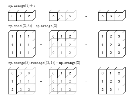
This image shows three examples of broadcasting. In the first, a scalar is added to a vector. In the second and third, arrays with compatible but different shapes are combined. NumPy virtually "stretches" the smaller arrays (shown as faded blocks) to match the larger array's shape before performing the element-wise operation.

Aggregations and the axis parameter

NumPy also provides fast aggregation functions like .sum(), .mean(), .max(), etc. When applied to a 2D array (a matrix), you can perform the aggregation over the entire matrix or along a specific dimension using the axis parameter. This is a critical concept.

• axis=0: Collapse along the rows (computes the aggregation for each column).
• axis=1: Collapse along the columns (computes the aggregation for each row).

Let's see this in action:

matrix = np.array([
    [1, 2, 3],
    [4, 5, 6]
])

# Sum of all elements
print(f"Total sum: {matrix.sum()}")  # Output: 21

# Sum along axis=0 (sum of each column)
print(f"Column sums: {matrix.sum(axis=0)}") # Output: [5 7 9]
# (1+4=5, 2+5=7, 3+6=9)

# Sum along axis=1 (sum of each row)
print(f"Row sums: {matrix.sum(axis=1)}")   # Output: [ 6 15]
# (1+2+3=6, 4+5+6=15)

Mastering the axis parameter is essential for many data manipulation tasks in machine learning.

Indexing and Slicing

Accessing elements in NumPy arrays is similar to Python lists, but with extensions for multiple dimensions.

Here's a summary of indexing techniques:

• Basic Indexing: A[row, col] to get a single element.
• Slicing: A[start_row:end_row, start_col:end_col] to get a sub-matrix.
• Boolean Indexing: A[A > 5] to get all elements in A that are greater than 5. This returns a 1D array.

A = np.array([
    [1, 2, 3, 4],
    [5, 6, 7, 8],
    [9, 10, 11, 12]
])

# Get the element at row 1, column 2
print(A[1, 2]) # Output: 7

# Get the first two rows and columns 1 through 2
# Rows 0 and 1, Columns 1 and 2
print(A[0:2, 1:3])
# Output:
# [[2 3]
#  [6 7]]

# Get all elements greater than 8
print(A[A > 8]) # Output: [ 9 10 11 12]

A Practical Example: Image Manipulation

To see how these concepts come together, let's look at a practical application that should resonate with your background in EEE and linear algebra: image manipulation. A color image can be represented as a 3D NumPy array with shape (height, width, 3), where the last dimension holds the Red, Green, and Blue (RGB) color channels.

The following tutorial uses the Singular Value Decomposition (SVD) to compress an image, but we'll just focus on the initial setup, which perfectly illustrates vectorized operations on a multi-dimensional array.

The line img_gray = img_array @ [0.2126, 0.7152, 0.0722] is a beautiful demonstration of vectorization. Here, img_array has shape (768, 1024, 3) and the list [0.2126, 0.7152, 0.0722] is a vector of weights. The @ operator performs matrix multiplication. NumPy broadcasts this operation across all 768 * 1024 pixels. For each pixel, it multiplies the [R, G, B] vector by the weight vector to produce a single grayscale intensity value.

This single line of code replaces a nested for loop that would iterate over every pixel's height and width. It's concise, readable, and executes at near-C speed. This is the paradigm you will use throughout your machine learning journey.

Conclusion

In this lesson, you've been introduced to NumPy, the workhorse of numerical computation in Python. We've moved beyond simple Python lists to a data structure that is purpose-built for the kind of high-performance math that machine learning demands.

Here are the key takeaways:

• NumPy's ndarray is a fast, memory-efficient grid of homogeneous data.
• Vectorization is the practice of applying operations to entire arrays at once, which is drastically faster than using Python loops due to low-level optimizations and parallel processing capabilities.
• Broadcasting provides a flexible way to perform operations on arrays of different, but compatible, shapes.
• Key tools for array manipulation include multi-dimensional indexing/slicing, aggregation functions (sum, mean), and the axis parameter for controlling the dimension of an operation.

You now have the tools to handle numerical data efficiently. In the next lesson, we will build directly on this foundation by introducing Pandas. Pandas uses NumPy arrays under the hood but provides a more powerful and convenient structure called a DataFrame for working with labeled, tabular data—the format you'll encounter most often in real-world datasets.