Loading and Inspecting DataFrames from CSVs

From NumPy Arrays to Pandas DataFrames

Imagine a spreadsheet. It has rows and columns, and each column has a name (a label). The columns can hold different types of data: one column for names (text), another for age (integers), and another for salary (floating-point numbers). A Pandas DataFrame is the programming equivalent of this concept.

A DataFrame is a two-dimensional, size-mutable, and potentially heterogeneous tabular data structure with labeled axes (rows and columns).

To build an intuition for this structure, it's helpful to relate it to a standard Python dictionary. The following video by Corey Schafer provides an excellent explanation of how a DataFrame can be thought of as a dictionary of lists, where the keys are the column names and the lists are the column values.

As you saw, you can create a DataFrame directly from a dictionary. The keys become the column headers, and the lists of values become the columns.

import pandas as pd

# A dictionary where keys are column names and values are the data in those columns
people_data = {
    'first_name': ['Corey', 'Jane', 'John'],
    'last_name': ['Schafer', 'Doe', 'Doe'],
    'email': ['CoreyMSchafer@gmail.com', 'JaneDoe@email.com', 'JohnDoe@email.com']
}

# Create a DataFrame from the dictionary
df = pd.DataFrame(people_data)

# Display the DataFrame
print(df)

This would output:

  first_name last_name                  email
0      Corey   Schafer  CoreyMSchafer@gmail.com
1       Jane       Doe        JaneDoe@email.com
2       John       Doe        JohnDoe@email.com

While creating DataFrames manually is useful, in machine learning, you will almost always load data from an external file. The most common format for this is the CSV (Comma-Separated Values) file.

Loading Data with pd.read_csv()

A CSV file is a simple text file where values are separated by commas, representing the columns of a table. Pandas provides a powerful and flexible function, pd.read_csv(), to load data from these files directly into a DataFrame.

This function can read files from your local computer or even directly from a URL on the internet. Let's explore how it works.

The ability to load data from a URL is extremely useful. Let's try it with the famous Iris dataset, a classic dataset in machine learning.

import pandas as pd

# The URL for the raw Iris dataset CSV file
url = 'https://archive.ics.uci.edu/ml/machine-learning-databases/iris/iris.data'

# The dataset doesn't have column names in the file, so we'll provide them.
column_names = ['sepal_length', 'sepal_width', 'petal_length', 'petal_width', 'class']

# Load the data from the URL into a DataFrame
iris_df = pd.read_csv(url, names=column_names)

# Now, iris_df is a Pandas DataFrame containing the data.

Your First Look at the Data: Basic Inspection

After loading a dataset, the very first task is to inspect it to understand its structure and content. You never want to start building a model without this initial reconnaissance. Pandas provides several essential attributes and methods for this.

A visual summary of some of the most common and useful attributes of a Pandas DataFrame. We will focus on shape, columns, and dtypes.

Let's go through the most critical inspection commands using our iris_df DataFrame.

1. Previewing the Data: .head()

The .head() method shows you the first 5 rows of the DataFrame. This is the quickest way to get a feel for the data and verify it loaded correctly.

# Display the first 5 rows
print(iris_df.head())

Output:

   sepal_length  sepal_width  petal_length  petal_width        class
0           5.1          3.5           1.4          0.2  Iris-setosa
1           4.9          3.0           1.4          0.2  Iris-setosa
2           4.7          3.2           1.3          0.2  Iris-setosa
3           4.6          3.1           1.5          0.2  Iris-setosa
4           5.0          3.6           1.4          0.2  Iris-setosa

2. Checking the Dimensions: .shape

The .shape attribute tells you the dimensions of the DataFrame as a (rows, columns) tuple. This should feel very familiar from your work with NumPy arrays.

# Get the shape of the DataFrame
print(iris_df.shape)

Output:

(150, 5)

This tells us our dataset has 150 rows (samples) and 5 columns (features).

3. Listing Column Names: .columns

The .columns attribute gives you the name of each column.

# Get the column names
print(iris_df.columns)

Output:

Index(['sepal_length', 'sepal_width', 'petal_length', 'petal_width', 'class'], dtype='object')

4. Checking Data Types: .dtypes

The .dtypes attribute is crucial. It shows the data type of each column. Just like in NumPy, operating on columns with the correct data type (int64, float64, etc.) is essential for performance and correctness. Text-based columns are typically represented with the object dtype.

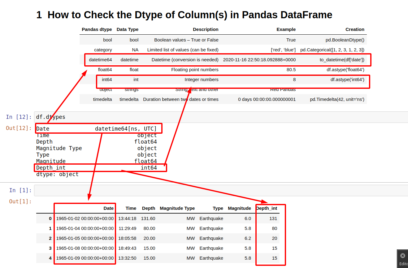
This image shows how the .dtypes attribute maps column names to their data types, such as int64 for integers and datetime64 for dates.

# Check the data types of each column
print(iris_df.dtypes)

Output:

sepal_length    float64
sepal_width     float64
petal_length    float64
petal_width     float64
class            object
dtype: object

We can see that the four measurement columns were correctly inferred as floating-point numbers, and the class column, containing the species name, is an object (string).

5. A Comprehensive Summary: .info()

Finally, the .info() method provides a concise summary of the DataFrame, including the index type, columns, non-null values, and memory usage. It's an incredibly efficient way to get a holistic view of your data.

# Get a full summary of the DataFrame
iris_df.info()

Output:

<class 'pandas.core.frame.DataFrame'>
RangeIndex: 150 entries, 0 to 149
Data columns (total 5 columns):
 #   Column        Non-Null Count  Dtype
---  ------        --------------  -----
 0   sepal_length  150 non-null    float64
 1   sepal_width   150 non-null    float64
 2   petal_length  150 non-null    float64
 3   petal_width   150 non-null    float64
 4   class         150 non-null    object
dtypes: float64(4), object(1)
memory usage: 6.0+ KB

The "Non-Null Count" column is particularly useful, as it gives you a quick way to spot columns with missing data. In this case, all columns have 150 non-null values, meaning our dataset is complete.

The following reading provides a great summary of these fundamental steps.

Conclusion

In this lesson, you've taken a major step from working with raw numbers in NumPy to handling structured, real-world data with Pandas. This marks the end of our foundational module on Python, and you are now equipped with the core programming tools for the rest of your machine learning journey.

Here are the key takeaways:

• A Pandas DataFrame is a 2D labeled data structure, like a spreadsheet, that holds columns of potentially different data types.
• You can load data from a CSV file into a DataFrame using the powerful pd.read_csv() function, which works with both local files and URLs.
• The first step after loading data is always inspection. The essential methods and attributes for this are:
  • .head() to preview the first few rows.
  • .shape to see the dimensions (rows, columns).
  • .columns to list the column names.
  • .dtypes to check the data type of each column.
  • .info() for a comprehensive summary.

You can now confidently load a dataset and understand its basic structure. In our next lesson, we will dive into the exciting world of data manipulation. You'll learn how to select specific rows and columns and filter your data based on conditions, allowing you to start asking meaningful questions and extracting insights.