Hello! In our previous lessons, we've established the foundational components of Azure Monitor. We explored the dual data platform of metrics and logs and then dove into Application Insights, seeing how it collects rich telemetry—requests, dependencies, exceptions, and traces—from your applications. All of this invaluable data is ultimately stored in a Log Analytics workspace.
Today, we'll learn how to unlock the insights hidden within that data. Our goal is to formulate basic queries using Kusto Query Language (KQL) to analyze operational data in Log Analytics. As a software architect, your ability to quickly and effectively query operational data is not just a troubleshooting skill; it's a core competency for understanding system behavior, validating deployments, and making data-driven design decisions. KQL is the key that opens this door in the Azure ecosystem.
We'll start by understanding the philosophy behind KQL, particularly how its data-flow model differs from the declarative nature of SQL. Then, we will progressively build up your query skills, moving from simple filtering and projection to powerful aggregation and joining techniques that are essential for analyzing complex, distributed systems.
What is KQL? A Data-Flow Approach to Querying
Kusto Query Language (KQL) is a read-only language designed for exploring vast amounts of structured and semi-structured data. Its defining feature is a data-flow model, where a query is constructed as a pipeline of operations. The output of one operator becomes the input to the next, connected by the pipe character (|).
This is a fundamental departure from SQL, where you typically declare what you want (e.g., SELECT col1, col2) before specifying where it comes from (FROM table). KQL follows a more intuitive investigative flow: start with a data source, then progressively filter, shape, and aggregate it.
The following article gives an excellent overview of KQL and its core differences from SQL. As someone with a strong engineering background, you'll find the comparison of their underlying models particularly relevant.
What is Kusto Query Language (KQL) - Pluralsight
This Pluralsight article provides a solid introduction to KQL's purpose and structure, with a direct comparison to SQL that will be helpful for you.
Please read the following sections: Start with What is KQL? to understand the data-flow model. Next, review What is KQL used for? to see its applications in diagnostics and analytics. Finally, focus on the sections Transitioning from SQL to KQL. This part directly contrasts the two languages and provides context for why KQL was designed the way it was.
The key takeaway is that KQL is not a replacement for SQL, but a tool optimized for a different purpose: rapid, ad-hoc investigation and time-series analysis on telemetry data.
The Anatomy of a KQL Query
Let's start building some queries. The best way to learn is by doing. Microsoft provides a free Log Analytics demo environment that we will use throughout this lesson. You can access it at https://aka.ms/lademo.
In the following video, John Savill provides an excellent hands-on tour of KQL fundamentals using a similar demo environment. We'll watch it in segments as we build up our skills.
Kusto Query Language (KQL) Overview
John Savill's technical training on KQL provides a clear and practical demonstration of the core operators. We'll start with the basics of scoping, filtering, and shaping data.
Watch the segment from the first query. Pay attention to: The basic structure: TableName | operator. Using take to get a sample of data without running a costly full-table query. Using project to select specific columns, similar to SELECT in SQL. Renaming columns with project (e.g., Description = StormSummary.Details.Description). Filtering data with where and interacting with semi-structured JSON data.
Let's formalize those core operators:
- Source: Every query starts with a table name (e.g.,
SecurityEvent,Perf,Requests). take <number>: Returns an arbitrary set of records. Essential for quickly inspecting a table's schema and data without a full scan.where <condition>: Filters the data. This is the most important operator for performance. As a best practice, always filter by time first if possible (e.g.,where TimeGenerated > ago(7d)).project <columns>: Selects the columns to include in the output. You can also rename columns (MyColumn = a.b.c) and remove columns (project-away <column_to_remove>).
A common mistake for beginners is to pull all data and then filter. KQL's optimizer is smart, but it's most effective when you tell it to narrow the dataset as early as possible.
Recon your Azure resources with Kusto Query Language (KQL)
This short clip from KnowOps gives two critical performance tips that are essential for writing efficient queries.
Watch the section on performance optimization tips. The advice to filter by timestamp first and project only needed columns is fundamental.
Aggregating Data with summarize
Filtering and projecting are useful, but the real power of KQL comes from aggregation. The summarize operator allows you to group rows and compute aggregate functions, similar to SQL's GROUP BY.
This is how you turn millions of raw log entries into meaningful statistics, like error counts per hour, average request duration by service, or the number of failed logins per computer.
Let's return to John Savill's video to see summarize in action, along with another useful operator, extend.
Kusto Query Language (KQL) Overview
This next segment demonstrates how to aggregate data and create new, calculated columns in your dataset.
Watch from the summarize operator. Focus on: Using summarize with an aggregate function like count() and grouping it with by EventType. Using extend to create a new calculated column (like Duration = EndTime - StartTime) without removing the original columns. Chaining operators to filter, summarize, and then filter the aggregated results again.
The pattern summarize <aggregation> by <grouping_column> is one you will use constantly. Some common aggregation functions include:
count(): Number of rows in the group.dcount(column): Approximate count of distinct values in a column.avg(column),sum(column),min(column),max(column): Standard mathematical aggregates.arg_max(column_to_maximize, column_to_return): Finds the row with the maximum value in one column and returns the value of another column from that same row. Extremely useful for "find the latest" scenarios.
Visualizing Query Results
Once you've aggregated your data, a table of numbers is often not the most intuitive way to understand it. KQL includes a render operator that can instantly turn your query results into charts.
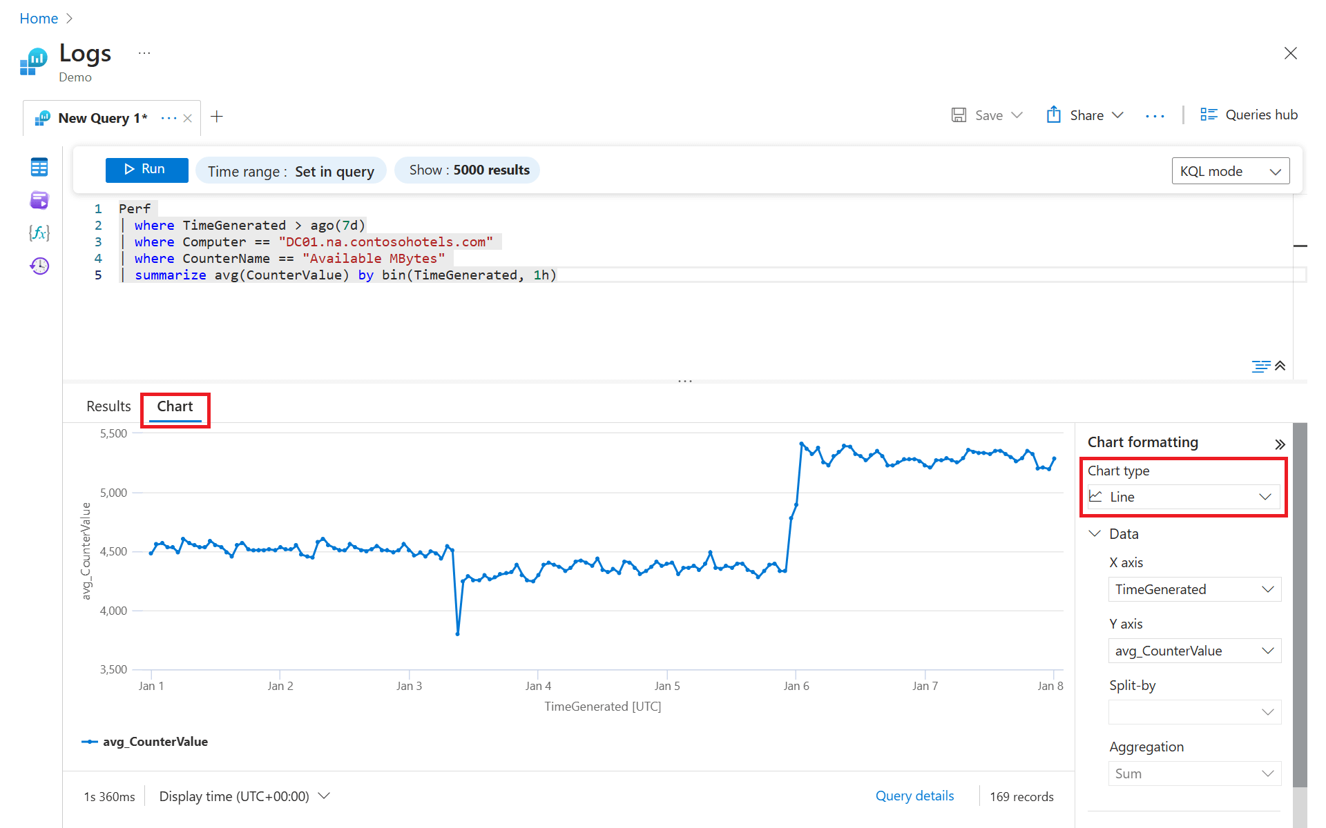
This is not just a UI feature; you can specify the visualization as the final step in your query pipeline.
Kusto Query Language (KQL) Overview
Let's see how easy it is to add visualization directly to your queries.
Watch this short segment on the render operator. You'll see how a simple | render piechart can transform your data into an actionable insight.
The most common render types are timechart, barchart, and piechart. This capability allows you to build simple dashboards and reports directly within the Log Analytics interface.
Combining Data with join
Distributed systems generate data in different tables. Application requests might be in the requests table, performance counters in Perf, and security logs in SecurityEvent. To get a complete picture, you need to combine these datasets. The join operator is how you achieve this.
Given your background, you're familiar with SQL joins. KQL's join is conceptually similar but with a syntax that fits the pipeline model. The different join kinds (inner, outer, anti) are critical for architectural analysis.
Kusto Query Language (KQL) Overview
This final segment from John Savill's tutorial provides one of the clearest explanations of KQL joins available. He methodically covers the different join kinds and their use cases.
Please watch the entire segment on joining multiple tables. Pay close attention to: The basic syntax: left_table | join kind=<kind> (right_table) on <attribute>. The difference between the default innerunique and the more common inner. The behavior of leftouter for finding all items on the left side, even if they have no match on the right. The explicit syntax for joining on columns with different names: on $left.columnA == $right.columnB.
Understanding the different join kinds is crucial. For example, using a leftanti join between a table of all expected VMs and a table of heartbeats is a powerful way to find which VMs are not reporting in.
A Practical Example: Finding Vulnerable Servers
Let's put everything together with a realistic query. An important operational and security task is to identify systems that have been running for a long time without a reboot, as they are more likely to be unpatched and vulnerable. This query against the Perf table does exactly that.
Recon your Azure resources with Kusto Query Language (KQL)
This final example from KnowOps demonstrates a sophisticated query that combines multiple operators to solve a real-world problem.
Watch this advanced example on finding long-running servers. Notice how it combines: where clauses with or to filter for uptime counters from both Windows and Linux. extend to compute a new uptime column from raw counter values. summarize arg_max(TimeGenerated, *) by Computer to get only the single latest record for each computer. This is a very common and powerful pattern. order by uptime desc to sort the most vulnerable servers to the top.
This single query demonstrates the power of KQL to transform raw telemetry into prioritized, actionable intelligence—a key skill for anyone in a senior engineering or architectural role.
Conclusion
In this lesson, we've moved from data collection to data analysis, equipping you with the fundamental skills to query operational data in Azure using KQL. You now have the tools to ask complex questions of your systems and get answers quickly.
Key Takeaways:
- KQL is a data-flow language: Its pipeline model (
|) is intuitive for exploratory analysis. - The core query structure is to filter, shape, and aggregate:
- Filter with
where, especially onTimeGenerated. - Shape results with
projectandextend. - Aggregate with
summarizeto turn raw data into statistics.
- Filter with
- Performance is key: Filter as early as possible and project only the columns you need.
joinis essential for correlating data from different sources, and understanding thekindis critical for correct analysis.renderallows for quick visualization of query results directly in Log Analytics.
You can now write queries to find specific errors, calculate performance baselines, and identify operational anomalies. The next logical step is to automate this detection. In our next lesson, we will learn how to design an alerting strategy using Azure Monitor action groups and alert rules, turning your KQL queries into a proactive monitoring system.