Welcome to our fifth lesson. In the previous lesson, we delved into the Central Limit Theorem, which explained how the sum of many independent random variables converges to a Gaussian distribution. This was our first formal encounter with the powerful idea that macroscopic regularity emerges from microscopic randomness in the asymptotic limit of large numbers.
Today, we will develop another essential asymptotic tool, one that is indispensable for moving from probability theory to statistical mechanics. Our objective is to learn how to evaluate integrals asymptotically using the saddle-point (or steepest descent) approximation. You will frequently encounter integrals in statistical mechanics, particularly when calculating partition functions, which involve summing or integrating over all possible microstates of a system. These integrals are typically high-dimensional and impossible to solve exactly. The saddle-point method provides a systematic way to find an excellent approximation in the thermodynamic limit (i.e., for a large number of particles, ).
1. From Real Peaks to Complex Saddles: The Intuition
Let's begin with a simpler, one-dimensional version of the problem known as Laplace's Method. Consider an integral of the form:
where is a large positive parameter. The intuition here is straightforward. The exponential function will be overwhelmingly dominated by the value of where attains its maximum. If this maximum occurs at a single point within the interval , then the function will look like an extremely sharp peak centered at . The entire value of the integral comes from the immediate vicinity of this peak.
This suggests we can approximate the integral by:
- Expanding in a Taylor series around its maximum . Since is a maximum, and . The expansion is .
- Approximating the slowly varying function by its value at the peak, .
- Extending the integration limits from to , since the contribution from outside the peak's neighborhood is negligible.
This transforms the original integral into a Gaussian integral, which we can solve exactly. The following reading from a University of Cambridge course on Asymptotic Methods formalizes this argument.
[PDF] ASYMPTOTIC METHODS - DAMTP
These notes provide a concise mathematical derivation of Laplace's method.
Please read the section titled "Laplace's Integral with Interior Maximum". This section will walk you through the steps of Taylor expanding the exponent and performing the resulting Gaussian integral to arrive at the leading-order asymptotic formula.
As the notes demonstrate, this procedure yields the standard formula for Laplace's method:
This result is foundational. Now, what happens if the function in the exponent is complex? This is where we generalize from Laplace's method on the real line to the method of steepest descent in the complex plane.
2. The Method of Steepest Descent: A Complex Generalization
Let's consider an integral along a contour in the complex plane:
Here, is a complex variable, and is an analytic function. Let's write in terms of its real and imaginary parts: , where . The integral becomes:
This integrand has both a rapidly varying magnitude (from ) and a rapidly oscillating phase (from ). The method of steepest descent offers a brilliant strategy to handle this.
The core idea is to use Cauchy's integral theorem, which states that we can deform the integration contour without changing the value of the integral, as long as we don't cross any singularities of the integrand. The "trick" is to deform the original contour to a new one, , along which the imaginary part of is constant, i.e., .
Professor Steven Strogatz provides an exceptionally clear explanation of this strategy.
In this video, Prof. Strogatz introduces the method of steepest descent and its core strategy.
Please watch from the beginning of the lecture up to the end of the strategy overview. Pay close attention to how deforming the contour to a path of constant imaginary part transforms the problem into a form that is amenable to Laplace's method.
If we can find such a path where , the rapidly oscillating term becomes a constant that can be pulled outside the integral. We are then left with:
This is now a purely Laplace-type integral, where the value is determined by the maximum of the real function along the new path. This elegant maneuver converts a difficult problem in the complex plane into a more manageable real-variable problem.
3. Why "Steepest Descent"?
You might be wondering about the name of the method. Why is a path of "constant imaginary part" called a path of "steepest descent"? This connection is a beautiful consequence of the properties of analytic functions, which you've encountered in your mathematical physics courses.
For an analytic function , the Cauchy-Riemann equations hold: and . A direct consequence of this is that the gradient vectors of the real and imaginary parts are orthogonal: .
From multivariable calculus, we know two things:
- The gradient points in the direction of the fastest increase of . Consequently, is the direction of steepest descent.
- The gradient is always perpendicular to the level curves of (curves where is constant).
Since , the direction of steepest descent for must be parallel to the level curves of . Therefore, a path of constant imaginary part () is precisely a path of steepest descent for the real part ().
This is where the method gets its name. We deform our contour onto a path that descends as steeply as possible from a "mountain pass" or saddle point. A saddle point is a point where the function is stationary, i.e., . At this point, both and . These are the points from which paths of steepest descent originate.
The following video section and notes offer excellent visualizations of this geometric relationship.
Prof. Strogatz continues his lecture to explain this geometric connection.
Watch the segment from "Why is this method called steepest descent?". The example with \phi(t) = t^2 and the orthogonal families of hyperbolas provides a concrete picture of this principle.
The ECE lecture notes below provide static diagrams that are also very helpful for visualizing the "landscape" around a saddle point.
[PDF] Notes 15 6382 Steepest-Descent Method.pdf
These notes offer a highly visual, step-by-step breakdown of the method.
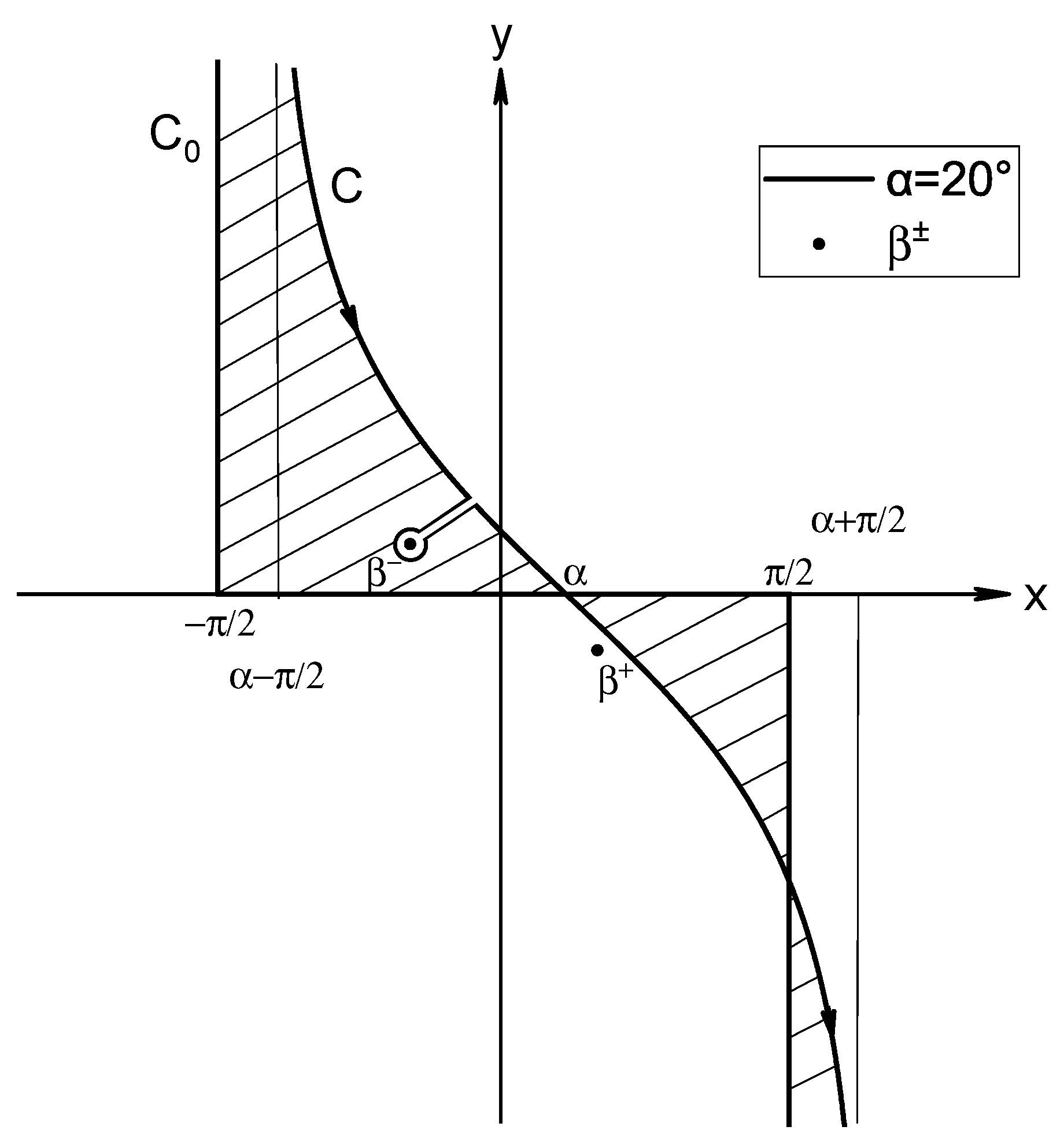
Skim through pages 6 to 19 (pages 6-19) to see the diagrams illustrating the saddle shape of the function u(x,y) and how the path of steepest descent (SDP) and steepest ascent (SAP) are defined relative to it. Notice the proof on page 19 showing \nabla u \perp \nabla v.
4. The Saddle-Point Formula and Stirling's Approximation
With the geometric intuition in place, we can state the main result. We approximate the integral by expanding around the saddle point , just as in Laplace's method:
The integral along the steepest descent path then becomes a Gaussian integral in the complex plane, leading to the final formula:
This looks just like the Laplace formula, but one must be careful with the phase of the complex number inside the square root. The choice of path direction resolves this ambiguity.
A classic and essential application of this method is the derivation of Stirling's formula, an approximation for the Gamma function for large .
We start with the integral representation of the Gamma function:
To put this into the standard form, we can write . The integral is . This isn't quite due to the lone . We perform a change of variables , which gives:
Now the integral is in the perfect form for the saddle-point approximation, with and . Since the integrand is real, this is technically an application of Laplace's method, but it follows the same logic.
The following resource provides a clear derivation.
[PDF] Notes 15 6382 Steepest-Descent Method.pdf
This section of the notes works through the derivation of Stirling's formula step-by-step.
Please study the example on pages 44-47, which starts with the Gamma function. Follow the identification of \phi(z), the calculation of the saddle point (z_0=1), and the evaluation of the derivatives at that point to arrive at the final formula.
By applying the saddle-point formula, we arrive at the celebrated Stirling's approximation:
This formula is ubiquitous in statistical mechanics for dealing with the factorials that arise from counting states (e.g., in Boltzmann's entropy formula).
5. A Complete Example: Beyond Stationary Phase
The real power of the method shines when the original contour is not the steepest descent path and must be deformed. This often allows for the calculation of higher-order terms in the asymptotic expansion that simpler methods miss.
Professor Strogatz's video works through a fantastic example, . The simpler method of stationary phase would give the leading-order term but would be unable to find the next term in the expansion. Steepest descent can find the full series. The process involves:
- Identifying the paths of constant imaginary part.
- Noting that the endpoints (0 and 1) lie on paths with different constant phase.
- Constructing a new, three-part contour: a path from the origin, a path into the endpoint at 1, and a "bridge" connecting them at infinity.
- Showing that the contribution from the bridge vanishes.
- Calculating the contributions from the two remaining paths. The path from the origin gives the stationary phase result (), and the path into the endpoint gives the next-order correction ().
This is an advanced application, but watching the derivation is extremely instructive.
This long segment contains the full, detailed worked example.
Watch from the start of the example to its conclusion. The key is not to memorize every algebraic step, but to follow the overarching logic: constructing the contour, justifying its pieces, and then applying Laplace's method to each contributing part. This demonstrates the full power and art of the technique.
Conclusion
In this lesson, we have added the saddle-point method to our arsenal of asymptotic techniques. It is a cornerstone of theoretical physics, allowing us to approximate the complex integrals that define partition functions and other key quantities in statistical mechanics.
Key Takeaways:
- The saddle-point (or steepest descent) method is a powerful technique for asymptotically evaluating integrals of the form for large .
- The method relies on deforming the integration contour in the complex plane to a path of steepest descent for the real part of .
- This path is equivalent to a path of constant imaginary part, which simplifies the integral by factoring out the oscillatory component.
- The dominant contribution to the integral comes from the neighborhood of saddle points, where .
- The method provides not just the leading-order behavior but can be used to generate a full asymptotic series, as exemplified by Stirling's formula for .
In the last lesson of this introductory module, we will explore the Large Deviation Principle. You'll find that the function we analyzed today, which determines the peak of the integrand, is deeply connected to the "rate function" in large deviation theory, which quantifies the probability of rare events in macroscopic systems.