Central Limit Theorem for Sums of Independent Random Variables

Welcome to our fourth lesson. Last time, we developed a powerful mathematical toolkit centered on moment-generating and characteristic functions. We saw that the logarithm of a characteristic function—the cumulant-generating function—is particularly useful because its Taylor series coefficients are the cumulants, which are additive for independent random variables. We also established that the Gaussian distribution is unique in that all its cumulants beyond the second (the variance) are zero.

This lesson builds directly on that foundation to explore one of the most profound and far-reaching results in probability theory and statistical physics. Our goal is to derive and apply the central limit theorem (CLT) to sums of independent random variables. You will see why the Gaussian distribution appears so ubiquitously, from experimental error analysis to the fluctuations of macroscopic quantities. The CLT provides the crucial link between the chaotic, random behavior of microscopic constituents and the predictable, deterministic laws that govern macroscopic systems.

1. The Emergence of Order: Motivating the Central Limit Theorem

Macroscopic observables in physics, like the total energy or magnetization of a material, are typically sums over a vast number of microscopic contributions. Let's consider a sum of $N$ independent and identically distributed (i.i.d.) random variables, $S_{N} = X_{1} + X_{2} + \dots + X_{N}$ .

How does this sum behave as $N$ becomes large? From the properties of cumulants we studied, we know that the mean and variance are extensive:

Mean: $⟨ S_{N} ⟩ = N ⟨ X ⟩$
Variance: $Var (S_{N}) = N \cdot Var (X)$

The variance, and thus the standard deviation $σ_{S_{N}} = N σ_{X}$ , grows with $N$ . This means the probability distribution of $S_{N}$ becomes wider and wider, never converging to a fixed shape.

What if we consider the sample mean, $X ˉ_{N} = S_{N} / N$ ? Its variance is $Var (X ˉ_{N}) = Var (X) / N$ , which goes to zero as $N \to \infty$ . The distribution of the sample mean collapses to a single point—a degenerate and rather uninteresting limit. This is the essence of the Law of Large Numbers.

This suggests that to find a non-trivial limiting distribution, we need to scale the sum differently. The "sweet spot" is to scale the sum in a way that keeps its variance constant. Since $Var (S_{N}) \propto N$ , dividing $S_{N}$ by $N$ should do the trick. The following video from MIT OpenCourseWare provides an excellent conceptual introduction to this scaling argument.

L19.2 The Central Limit Theorem

This video brilliantly explains the motivation behind the specific scaling used in the Central Limit Theorem.

Watch the video from the beginning until the formal statement. Pay close attention to the three cases the lecturer presents: The sum S_N, whose distribution spreads out. The sample mean S_N/N, whose distribution collapses. The appropriately scaled sum S_N/\sqrt{N}, whose variance remains constant, allowing it to approach a non-trivial shape.

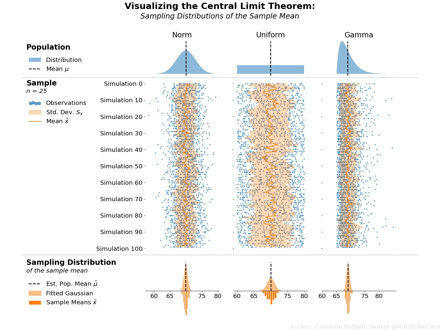
As the video explains, the correct variable to study is the standardized sum. If each $X_{i}$ has mean $μ$ and variance $σ^{2}$ , the standardized sum is:

Z_{N} = \frac{S _{N} - ⟨ S _{N} ⟩}{Var ( S _{N} )} = \frac{\sum _{i = 1}^{N} X _{i} - N μ}{σ N}

By construction, $Z_{N}$ has a mean of 0 and a variance of 1 for any $N$ . The Central Limit Theorem states that as $N \to \infty$ , the probability distribution of $Z_{N}$ converges to the standard normal (Gaussian) distribution, regardless of the distribution of the individual $X_{i}$ .

This figure provides a powerful analogy from signal processing. The probability density function of a sum of two independent random variables is the convolution of their individual PDFs. This image shows that repeatedly convolving an arbitrary initial signal (a) results in a signal that rapidly approaches a Gaussian shape (c). This is the visual counterpart to the mathematical mechanism behind the CLT.

This visualization demonstrates the universality of the CLT. For three different underlying population distributions (Normal, Uniform, and Gamma), 100 simulations of drawing a sample of size n=25 are shown. The bottom row plots the distribution of the 100 sample means ($\bar{X}$) for each case. Despite the drastic differences in the original populations, the sampling distribution of the mean is remarkably Gaussian in all three cases.

2. A Rigorous Derivation of the Central Limit Theorem

Having established the intuition, we will now derive the theorem with the rigor you appreciate. The proof elegantly combines the properties of characteristic functions and cumulants from our previous lesson. The core strategy is to find the characteristic function of the standardized sum $Z_{N}$ and show that, in the limit $N \to \infty$ , it becomes the characteristic function of the standard normal distribution, which we know is $ϕ_{N (0, 1)} (k) = e^{- k^{2} /2}$ . By Lévy's continuity theorem, convergence of characteristic functions implies convergence of the distributions.

You can follow the full, rigorous argument in the following lecture notes. I will outline the key steps below.

[PDF] 18.600: Lecture 30 .1in Central limit theorem

These notes from an MIT probability course provide a concise and elegant proof of the CLT using characteristic functions.

First, review the section on characteristic functions and Lévy's continuity theorem. This theorem is the formal justification for our proof strategy. Next, work through the proof itself. The logic is almost identical to the MGF proof presented just before it, but uses characteristic functions, making it more general.

Let's walk through the logic of the proof presented in the notes.

Standardize the Variables: It's easier to work with variables that have zero mean and unit variance. Let's define $Y_{i} = (X_{i} - μ) / σ$ . Each $Y_{i}$ is an i.i.d. random variable with $⟨ Y_{i} ⟩ = 0$ and $Var (Y_{i}) = 1$ . The standardized sum can then be written as $Z_{N} = \frac{1}{N} \sum_{i = 1}^{N} Y_{i}$ .
Characteristic Function of the Sum: Let $ϕ_{Y} (k) = ⟨ e^{ik Y} ⟩$ be the characteristic function of a single $Y_{i}$ . Using the properties of characteristic functions for sums of independent variables and for scaled variables, the characteristic function of $Z_{N}$ is:
$ϕ_{Z_{N}} (k) = ⟨ exp (ik \frac{1}{N} i \sum Y_{i}) ⟩ = [ϕ_{Y} (\frac{k}{N})]^{N}$
Cumulant Expansion: Now we use the tool from our last lesson: the logarithm of the characteristic function, which generates the cumulants. Let's Taylor expand $ln ϕ_{Y} (t)$ for small $t$ :
$ln ϕ_{Y} (t) = m = 1 \sum \infty \frac{( i t ) ^{m}}{m !} ⟨ Y^{m} ⟩_{c}$
We know the first two cumulants of our standardized variable $Y$ :
- $⟨ Y^{1} ⟩_{c} = ⟨ Y ⟩ = 0$
- $⟨ Y^{2} ⟩_{c} = Var (Y) = 1$
  So, the expansion becomes:
$ln ϕ_{Y} (t) = 0 \cdot (i t) + \frac{( i t ) ^{2}}{2 !} \cdot 1 + O (t^{3}) = - \frac{t ^{2}}{2} + O (t^{3})$
Take the Limit: Substitute this expansion back into our expression for $ϕ_{Z_{N}} (k)$ . We are interested in its logarithm:
$ln ϕ_{Z_{N}} (k) = N ln [ϕ_{Y} (\frac{k}{N})]$
Using our Taylor series with $t = k / N$ , we get:
$ln ϕ_{Z_{N}} (k) = N [- \frac{1}{2} (\frac{k}{N})^{2} + O ((\frac{k}{N})^{3})]$ $ln ϕ_{Z_{N}} (k) = N [- \frac{k ^{2}}{2 N} + O (\frac{k ^{3}}{N ^{3/2}})] = - \frac{k ^{2}}{2} + O (\frac{1}{N})$
In the limit as $N \to \infty$ , the higher-order term vanishes:
$N \to \infty lim ln ϕ_{Z_{N}} (k) = - \frac{k ^{2}}{2}$
Conclusion: Exponentiating both sides, we find that the characteristic function of $Z_{N}$ converges to the characteristic function of a standard normal random variable:
$N \to \infty lim ϕ_{Z_{N}} (k) = e^{- k^{2} /2}$
By Lévy's continuity theorem, this proves that $Z_{N}$ converges in distribution to $N (0, 1)$ .

The same logic can be found in a slightly different notation in the first MIT lecture notes resource, which you might also find illuminating.

[PDF] Statistical Mechanics I - MIT OpenCourseWare

This resource derives the CLT using the language of cumulants directly. It provides a complementary perspective to the characteristic function proof.

Read the section titled "Sums of Random Variables", and then focus on the argument starting from this paragraph. Notice how it explicitly shows that for the standardized variable y, the m-th cumulant scales as N^{1-m/2}, causing all cumulants for m > 2 to vanish as N \to \infty.

This alternative phrasing makes the key point explicit: in the thermodynamic limit, only the mean and variance matter for the collective fluctuations of the sum. The system "forgets" all other details (skewness, kurtosis, etc.) of the underlying microscopic probability distribution.

3. Application: The 1D Random Walk and Diffusion

To see the CLT in action, let's consider a classic problem from physics: the one-dimensional random walk. Imagine a particle on a line that starts at $x = 0$ . At discrete time steps, it moves a distance $l$ either to the left or to the right with equal probability.

Let the $i$ -th step be the random variable $x_{i}$ .

$x_{i} = + l$ with probability $p = 1/2$
$x_{i} = - l$ with probability $p = 1/2$

The properties of a single step are:

Mean: $μ = ⟨ x_{i} ⟩ = (+ l) \frac{1}{2} + (- l) \frac{1}{2} = 0$
Variance: $σ^{2} = ⟨ x_{i}^{2} ⟩ - μ^{2} = ((+ l)^{2} \frac{1}{2} + (- l)^{2} \frac{1}{2}) - 0 = l^{2}$

The position of the particle after $N$ steps is the sum $S_{N} = \sum_{i = 1}^{N} x_{i}$ . According to the CLT, for large $N$ , the distribution of $S_{N}$ will be approximately Gaussian. What are the parameters of this Gaussian?

Mean of sum: $⟨ S_{N} ⟩ = N μ = 0$
Variance of sum: $Var (S_{N}) = N σ^{2} = N l^{2}$

So, the probability density function for the particle's position $x$ after $N$ steps is approximately:

p (x, N) \approx \frac{1}{2 π N l ^{2}} exp (- \frac{x ^{2}}{2 N l ^{2}})

This result is profound. It's the fundamental solution to the diffusion equation, $\frac{\partial p}{\partial t} = D \frac{\partial ^{2} p}{\partial x ^{2}}$ , if we relate the number of steps $N$ to time $t$ and define a diffusion constant $D$ . The CLT provides a direct microscopic justification for the macroscopic phenomenon of diffusion. The root-mean-square displacement of the particle, $⟨ S_{N}^{2} ⟩ = N l^{2} = l N$ , grows with the square root of the number of steps (or time), a hallmark of diffusive processes.

Conclusion

Today, we have explored the Central Limit Theorem, a pillar of probability and statistical mechanics.

Key Takeaways:

The CLT states that the standardized sum of a large number of i.i.d. random variables converges to a standard normal (Gaussian) distribution, regardless of the original distribution, provided it has a finite variance.
The proof hinges on analyzing the characteristic function (or its logarithm, the CGF) of the standardized sum. A Taylor expansion shows that in the limit of a large number of terms, only the first two cumulants survive, which uniquely defines a Gaussian.
The theorem explains the ubiquity of the Gaussian distribution in nature and provides a fundamental justification for why the collective behavior of many random microscopic parts leads to simple, predictable macroscopic laws, such as diffusion.

The CLT is our first deep dive into the "asymptotic" world of large systems. In our next lesson, we will continue this theme by developing another indispensable tool for dealing with large $N$ : the saddle-point approximation (or method of steepest descent). This will allow us to evaluate the very large-dimensional integrals that arise when calculating partition functions in statistical mechanics.

Recommended resources

1. The Emergence of Order: Motivating the Central Limit Theorem

2. A Rigorous Derivation of the Central Limit Theorem

3. Application: The 1D Random Walk and Diffusion

Conclusion