Solving the 1D Ising Model with the Transfer Matrix Method

Introduction

In our last lesson, we critically examined mean-field theory and found its most glaring failure in one dimension. MFT incorrectly predicts a finite-temperature phase transition for the 1D Ising model, whereas physical arguments involving domain wall creation suggest that any amount of thermal energy is sufficient to destroy long-range order. This discrepancy highlights the danger of approximations that neglect fluctuations and motivates our turn towards an exact solution.

Today, we will derive that exact solution. The objective is to solve the 1D Ising model in zero magnetic field exactly using the transfer matrix method. This powerful technique, which you will encounter in various forms throughout statistical and quantum field theory, transforms a problem of summing over interacting degrees of freedom into a much simpler problem in linear algebra. By calculating the free energy exactly, we will rigorously prove the absence of a phase transition for $T > 0$ and lay the groundwork for calculating other exact quantities in the next lesson.

1. The Partition Function as a Matrix Product

Let's consider a one-dimensional chain of $N$ spins, where each spin $σ_{i}$ can be either +1 (up) or -1 (down). We'll assume periodic boundary conditions, meaning the chain is bent into a ring so that the $N$ -th spin interacts with the first. This arrangement is convenient as it makes every spin equivalent.

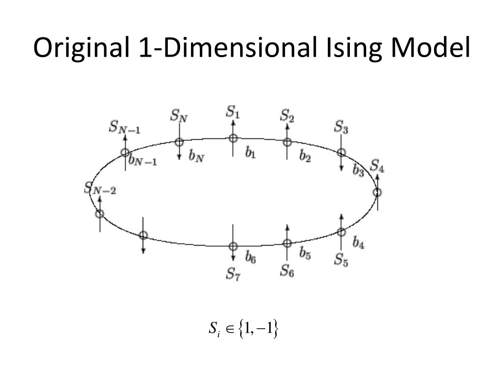
A one-dimensional chain of N spins, $\sigma_1, ..., \sigma_N$, arranged in a circle. The periodic boundary condition means that spin $\sigma_N$ is a neighbor of spin $\sigma_1$.

In the absence of an external magnetic field ( $h = 0$ ), the Hamiltonian for this system is given by the sum of nearest-neighbor interaction energies:

H = - J i = 1 \sum N σ_{i} σ_{i + 1}

Here, $J > 0$ corresponds to a ferromagnetic interaction, favoring aligned spins. The periodic boundary condition is enforced by setting $σ_{N + 1} \equiv σ_{1}$ .

Our goal is to compute the canonical partition function, which involves summing over all $2^{N}$ possible spin configurations:

Z_{N} = {σ_{1}, ..., σ_{N}} \sum e^{- β H} = σ_{1} = \pm 1 \sum \dots σ_{N} = \pm 1 \sum exp (β J i = 1 \sum N σ_{i} σ_{i + 1})

Directly evaluating this sum is computationally impossible for large $N$ . The key insight of the transfer matrix method is to rewrite the exponential of the sum as a product of exponentials:

Z_{N} = σ_{1} = \pm 1 \sum \dots σ_{N} = \pm 1 \sum i = 1 \prod N e^{β J σ_{i} σ_{i + 1}}

This expression looks like a sequence of matrix multiplications. To see this, let's define a 2x2 matrix $T$ whose elements connect the state of spin $σ_{i}$ to spin $σ_{i + 1}$ :

T_{σ_{i}, σ_{i + 1}} = e^{β J σ_{i} σ_{i + 1}}

Let's expand the sum for $Z_{N}$ to make the structure clear:

Z_{N} = σ_{1}, ..., σ_{N} \sum T_{σ_{1}, σ_{2}} T_{σ_{2}, σ_{3}} \dots T_{σ_{N - 1}, σ_{N}} T_{σ_{N}, σ_{1}}

Notice how the sum over $σ_{2}$ corresponds to the matrix multiplication of the first two $T$ matrices. Summing over all intermediate spins ( $σ_{2}, \dots, σ_{N}$ ) and finally over $σ_{1}$ to close the loop is equivalent to taking the trace of the $N$ -th power of the matrix $T$ .

The following video provides an excellent walkthrough of this "mathematical trickery," showing how the structure of the summation naturally leads to the trace of a matrix power.

The Ising model

This video by Gareth Tribello clearly explains the conceptual leap from a sum over spin configurations to the trace of a matrix product.

Please watch the segment from "From here on out". The key idea is to see how summing over an intermediate spin variable \sigma_i is equivalent to performing a matrix multiplication. Pay close attention to how the periodic boundary condition (\sigma_{N+1}=\sigma_1) naturally leads to the trace operation.

Having established this crucial connection, we can now write the partition function in a much more compact and powerful form:

Z_{N} = Tr (T^{N})

The matrix $T$ , known as the transfer matrix, has elements indexed by the possible spin values {+1, -1}:

T = (T_{1, 1} T_{- 1, 1} T_{1, - 1} T_{- 1, - 1}) = (e^{β J} e^{- β J} e^{- β J} e^{β J})

We have successfully converted a complex problem in statistical mechanics into a standard problem in linear algebra.

2. Diagonalization and the Free Energy

The trace of a matrix is invariant under a change of basis. If we diagonalize $T$ , the calculation of $T^{N}$ becomes trivial. Let $λ_{+}$ and $λ_{-}$ be the eigenvalues of $T$ . In the basis of its eigenvectors, $T$ is a diagonal matrix, and $T^{N}$ is simply the diagonal matrix of its eigenvalues raised to the power $N$ . Therefore:

Z_{N} = Tr (T^{N}) = λ_{+}^{N} + λ_{-}^{N}

Our next step is to find these eigenvalues. The following reading provides a concise and rigorous derivation.

[PDF] The Ising Model

This section from the textbook by Friedli and Velenik presents the formal proof of the exact solution for the 1D Ising model using the transfer matrix method.

Please read the "Proof of Theorem 3.9". This short section details the setup with periodic boundary conditions (on a torus), defines the transfer matrix A (which is our T), shows that Z = \text{Tr}(A^n), and calculates the eigenvalues. We are interested in the zero-field case, so you can set h=0 in their equations.

As shown in the text, the eigenvalues are found by solving the characteristic equation $det (T - λ I) = 0$ :

det (e^{β J} - λ e^{- β J} e^{- β J} e^{β J} - λ) = (e^{β J} - λ)^{2} - (e^{- β J})^{2} = 0

This gives $e^{β J} - λ = \pm e^{- β J}$ , leading to the two eigenvalues:

λ_{+} = e^{β J} + e^{- β J} = 2 cosh (β J)

λ_{-} = e^{β J} - e^{- β J} = 2 sinh (β J)

The partition function is therefore:

Z_{N} = (2 cosh (β J))^{N} + (2 sinh (β J))^{N}

Now, we take the thermodynamic limit, $N \to \infty$ . Since $cosh (x) > ∣ sinh (x) ∣$ for any real $x$ , the eigenvalue $λ_{+}$ is strictly larger than $λ_{-}$ for any finite temperature ( $β < \infty$ ). In the limit of large $N$ , the term $λ_{+}^{N}$ will completely dominate the sum.

Z_{N} = λ_{+}^{N} (1 + (\frac{λ _{-}}{λ _{+}})^{N}) \approx λ_{+}^{N} as N \to \infty

We can now calculate the Helmholtz free energy per spin, $f = F / N$ :

f = - \frac{1}{N} k_{B} T ln Z_{N} \approx - \frac{1}{N} k_{B} T ln (λ_{+}^{N}) = - k_{B} T ln (λ_{+})

Substituting the expression for $λ_{+}$ , we arrive at the exact free energy per spin for the 1D Ising model:

f (T) = - k_{B} T ln (2 cosh (β J)) = - k_{B} T ln (2 cosh (\frac{J}{k _{B} T}))

3. The Absence of a Phase Transition

This exact result holds the definitive answer to the question of a phase transition. In thermodynamics, a phase transition is signaled by a non-analyticity (a discontinuity, kink, or divergence) in the free energy or one of its derivatives with respect to temperature.

Let's examine our expression for $f (T)$ . The hyperbolic cosine function, $cosh (x)$ , is analytic for all real $x$ . The natural logarithm, $ln (y)$ , is analytic as long as its argument is positive. Since $cosh (J / k_{B} T) \geq 1$ for all $T$ , the argument $2 cosh (J / k_{B} T)$ is always positive and greater than or equal to 2.

Therefore, the function $f (T)$ is smooth and infinitely differentiable (analytic) for all temperatures $T > 0$ . There are no singularities, no discontinuities, and no cusps. This constitutes a rigorous proof that the one-dimensional Ising model has no phase transition at any finite, non-zero temperature.

At $T = 0$ ( $β \to \infty$ ), the system does order. We can see this by looking at the low-temperature limit of the free energy. For large $β J$ , $cosh (β J) \approx \frac{1}{2} e^{β J}$ , so:

f (T) \approx - k_{B} T ln (2 \cdot \frac{1}{2} e^{β J}) = - k_{B} T ln (e^{β J}) = - k_{B} T (β J) = - J

The energy per spin is $- J$ , which corresponds to the ground state where all spins are perfectly aligned. The order is destroyed as soon as $T$ becomes non-zero.

4. An Alternative Viewpoint: From Spins to Bonds

The transfer matrix method is a general and powerful tool. For the specific case of the 1D Ising model, there is an alternative and physically insightful way to arrive at the same result. This method, sometimes called a duality transformation, involves redefining the fundamental degrees of freedom from the spins $σ_{i}$ living on the sites to "bond" variables $τ_{i} = σ_{i} σ_{i + 1}$ living on the links between sites.

The following video by Leonard Susskind, part of which we saw in the previous lesson, develops this approach. It provides a beautiful illustration of how a seemingly complex problem of interacting spins can be mapped to a trivial problem of non-interacting bonds.

Statistical Mechanics Lecture 9

This segment of a Stanford lecture demonstrates an alternative solution to the 1D Ising model by transforming from spin variables to non-interacting bond variables.

Please watch from "trick the trick". The core idea is to change variables from spins \sigma_i to bond variables \mu_i = \sigma_i \sigma_{i+1}. The Hamiltonian becomes a simple sum over these independent bond variables, reducing the problem to that of a non-interacting paramagnet, which is easily solved. This elegant approach is mathematically equivalent to the transfer matrix method.

This change of variables makes it immediately obvious why the system is so simple: the interaction term $H = - J \sum_{i} σ_{i} σ_{i + 1}$ becomes $H = - J \sum_{i} τ_{i}$ . In this new representation, the Hamiltonian is just a sum over independent variables $τ_{i}$ , with no interactions between them. This is precisely the problem of an ideal paramagnet, which we know does not exhibit a phase transition.

Conclusion

In this lesson, we have confronted the failure of mean-field theory by deriving the exact solution for the one-dimensional Ising model. The transfer matrix method provided the crucial bridge, converting a statistical sum over $2^{N}$ configurations into the diagonalization of a simple 2x2 matrix.

Key Takeaways:

The partition function of a 1D chain with nearest-neighbor interactions and periodic boundary conditions can be expressed as the trace of the $N$ -th power of a transfer matrix, $Z_{N} = Tr (T^{N})$ .
In the thermodynamic limit ( $N \to \infty$ ), the partition function is dominated by the largest eigenvalue of the transfer matrix, $λ_{+}$ .
The free energy per spin is given by $f = - k_{B} T ln (λ_{+})$ . For the zero-field Ising model, this is $f (T) = - k_{B} T ln (2 cosh (J / k_{B} T))$ .
The exact free energy is analytic for all $T > 0$ , rigorously proving that the 1D Ising model does not have a finite-temperature phase transition.

We have now seen a powerful method for solving a model exactly. Having the exact free energy opens the door to calculating other physical observables with full precision. In our next lesson, we will use the transfer matrix framework to compute the spin-spin correlation function and the correlation length. This will provide a quantitative measure of how order decays with distance in the system and offer another point of stark contrast with the predictions of mean-field theory.

Recommended resources