Limitations of Mean-Field Theory

1. Confronting Reality: MFT vs. Exact Solutions

Mean-field theory's central prediction is a set of universal critical exponents, independent of the system's spatial dimension. Let's test this bold claim against what we know to be true from exact solutions.

The One-Dimensional Catastrophe

The simplest non-trivial interacting system is the 1D Ising model. While you have likely seen its solution via the transfer matrix method, the following video offers a brilliantly intuitive perspective on why it behaves the way it does. It explains how the problem can be cleverly mapped onto a system of non-interacting "bond" variables and uses the "game of telephone" analogy to explain the fate of correlations.

The key takeaways from the video are:

1. Exponential Decay of Correlations: The correlation between two spins separated by $n$ sites, $⟨{\sigma }_i{\sigma }_{i+n}⟩$, is proportional to $(\tanh (\beta J){)}^n$. Since $\tanh (\beta J)<1$ for any finite temperature $T>0$, this correlation decays exponentially to zero over a finite distance. The system has no "long-range memory."
2. No Finite-Temperature Phase Transition: A phase transition into an ordered state requires correlations to persist over infinite distances. Since this never happens for $T>0$, the 1D Ising model does not have a finite-temperature phase transition. The only ordered state is the ground state at $T=0$.
3. Energetic Argument: Creating a domain of flipped spins of any length in 1D costs a fixed, finite energy (associated with creating two domain walls at its ends). This finite energy cost cannot compete with the significant entropy gained by creating domains anywhere in the system.

This is a disastrous result for mean-field theory. Our MFT solution for the Ising model, $m=\tanh (2d\beta Jm)$, predicts a critical temperature $T_c=2dJ/k_B$. For $d=1$, this would be $T_c=2J/k_B>0$. Mean-field theory predicts a phase transition where one provably does not exist. It is not just quantitatively inaccurate; it is qualitatively wrong.

The Discrepancy in Higher Dimensions

Perhaps MFT fares better in higher dimensions. In 1944, Lars Onsager accomplished the monumental task of exactly solving the 2D Ising model. His solution revealed a finite critical temperature, confirming the intuition that higher dimensions can support an ordered phase. However, the critical exponents he found were starkly different from the mean-field values.

This is best seen in a direct comparison.

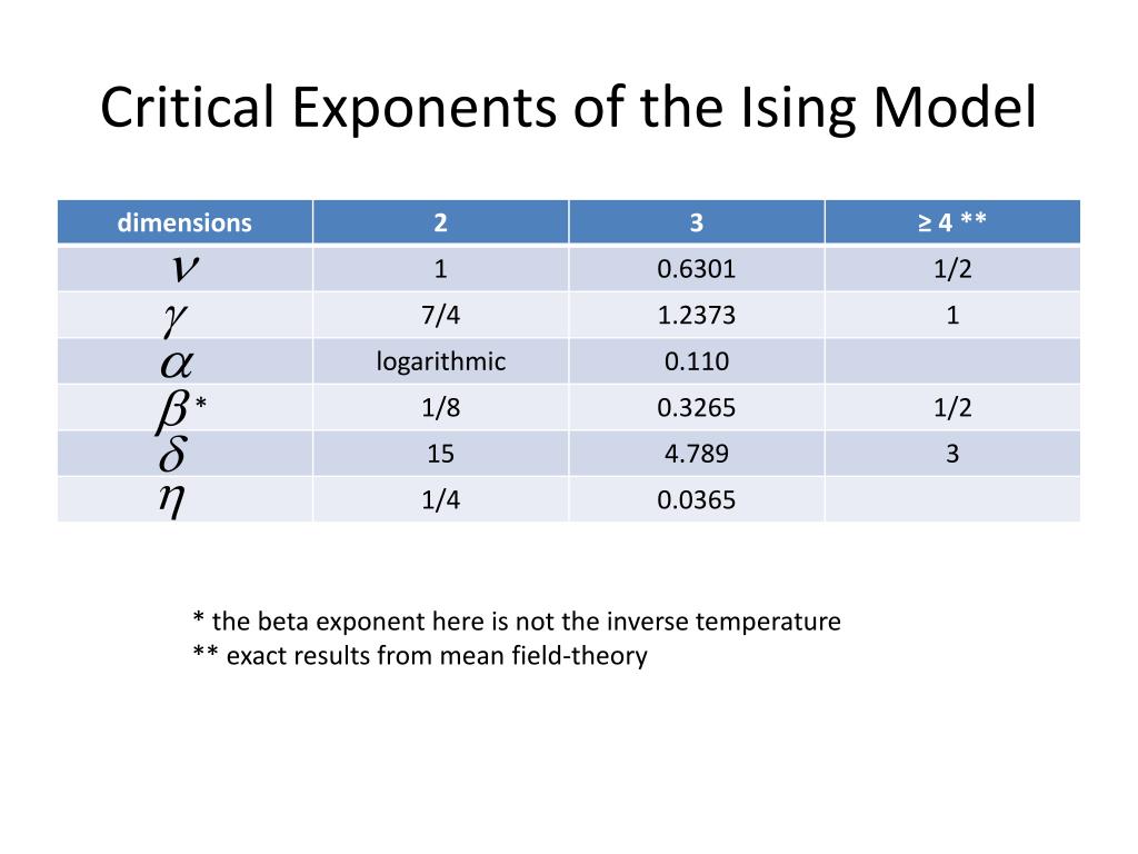
This table is profoundly illuminating.

• 2D: The exponents ($\beta =1/8,\gamma =7/4,\nu =1,\dots$) are completely different from the MFT values ($\beta =1/2,\gamma =1,\nu =1/2$). MFT is quantitatively wrong in 2D.
• 3D: High-precision numerical simulations (which for this problem are effectively exact) and experiments yield yet another set of exponents. They are closer to the MFT values than the 2D ones, but still distinctly different.
• $d\ge 4$: The table notes that for dimensions of 4 or greater, the exponents are indeed the exact mean-field values.

This leads to a crucial conclusion: Mean-field theory is an approximation that becomes exact only above a certain spatial dimension, known as the upper critical dimension, $d_u$. For the Ising universality class, $d_u=4$. Below this dimension, MFT fails because it neglects the very thing that determines the true critical behavior: fluctuations.

2. The Physics of Failure: Fluctuations and Dimensionality

The core assumption of MFT is the replacement of a fluctuating local environment with its static average. This simplification ignores the rich physics of correlated fluctuations, whose character is intimately tied to the system's dimensionality and symmetries.

The Domain Wall (Peierls) Argument

The energetic argument from Susskind's video can be generalized. This is a classic argument first advanced by Rudolf Peierls.

Consider a $d$-dimensional Ising system of linear size $L$ at low temperature, mostly in the "up" state. To destroy long-range order, the system must be able to spontaneously create domains of "down" spins. Let's weigh the free energy cost $\Delta F=\Delta E-T\Delta S$ of creating a single large domain that cuts across the system.

• Energy Cost ($\Delta E$): The domain is separated from the rest of the system by a "wall" of broken bonds. The area of this wall scales as $L^{d-1}$. The energy cost is therefore $\Delta E\propto J{L}^{d-1}$.
• Entropy Gain ($\Delta S$): The wall is not rigid; it can wobble and deform. The number of possible configurations for the wall gives it an entropy. A simple lower bound is that the wall can be shifted as a whole, giving an entropy that scales as $k_B\ln (L)$.

Comparing the two terms:

• For $d=1$, $\Delta E\propto J$ (constant) while $\Delta S\propto \ln (L)$. For a large system ($L\to \infty$), the entropy term will always win at any $T>0$. The system will fill with domain walls, destroying long-range order. We say the lower critical dimension for the Ising model is $d_{\ell }=1$.
• For $d>1$, $\Delta E\propto L^{d-1}$ grows much faster than $\Delta S\propto \ln (L)$. The large energy cost suppresses the formation of system-spanning domains, allowing the ordered phase to remain stable at low temperatures.

This simple argument beautifully explains why MFT's prediction of a phase transition fails for $d=1$ but holds qualitatively for $d>1$.

Continuous Symmetries and the Mermin-Wagner Theorem

The situation changes for systems with a continuous symmetry, like the XY model where spins are 2D vectors that can point in any direction in a plane. Here, the order parameter can change direction smoothly.

As the notes show, the gradual twist of the order parameter across the system corresponds to a low-energy Goldstone mode. The energy cost of such a twist scales not as $L^{d-1}$ but as ${\rho }_s{L}^{d-2}$, where ${\rho }_s$ is the spin stiffness.

Comparing this to the entropy gain ($\Delta S\propto \ln L$), we find that entropy wins for all $d\le 2$. This is the essence of the Mermin-Wagner theorem: spontaneous breaking of a continuous symmetry is forbidden in systems with short-range interactions for dimensions $d\le d_{\ell }=2$.

This means MFT, which would predict a phase transition for the XY model in $d=2$, is again qualitatively wrong. The fluctuations associated with the continuous symmetry are more effective at destroying order than those in the discrete Ising case, raising the lower critical dimension from 1 to 2. (Note: The 2D XY model does have a special kind of transition, the Kosterlitz-Thouless transition, but it is not associated with true long-range order).

3. The Quantitative Verdict: The Ginzburg Criterion

We now have a physical understanding of why MFT fails: fluctuations. But can we derive a condition that tells us precisely when it fails? This is the purpose of the Ginzburg criterion.

The idea is to use the Landau-Ginzburg free energy framework to estimate the contribution of fluctuations to a thermodynamic quantity (like the heat capacity) and compare it to the mean-field prediction. MFT will be valid as long as the fluctuation contribution is small.

The derivation leads to the Ginzburg criterion. It states that mean-field theory is a valid approximation only when the reduced temperature $t=|T-T_c|/T_c$ is much larger than a characteristic value, the Ginzburg reduced temperature $t_G$.

Here, $a$ is a microscopic length scale (like the lattice spacing), and ${\xi }_0$ is the correlation length at zero temperature. The region $|t|<t_G$ is the critical region, where fluctuations dominate and MFT is invalid.

This criterion elegantly explains the experimental situation:

• Conventional Superconductors: The ordered state consists of Cooper pairs, which are quantum mechanical objects with a very large size. The zero-temperature correlation length ${\xi }_0$ can be thousands of angstroms. With ${\xi }_0/a\sim 10^3$, the Ginzburg reduced temperature in $d=3$ is $t_G\sim (10^{-3}{)}^6=10^{-18}$. This critical region is so unimaginably narrow that no experiment can resolve it. Therefore, for all practical purposes, MFT (in the form of BCS theory) provides an excellent description all the way to $T_c$.

• Magnets, Liquid-Gas Transitions: In these systems, the fundamental constituents are atoms or localized spins. The correlation length ${\xi }_0$ is on the order of the inter-atomic spacing $a$. This means ${\xi }_0/a\sim 1$, which makes $t_G\sim 1$. The critical region is enormous. MFT fails as soon as the system begins to feel the effects of the critical point.

The Ginzburg criterion provides the final piece of the puzzle. It not only confirms that MFT fails due to fluctuations but gives us a powerful, predictive tool to estimate the size of the temperature window where this failure occurs. It reinforces the concept of the upper critical dimension $d_u=4$, since the exponent in the expression for $t_G$ diverges as $d\to 4$, indicating that for $d\ge 4$, MFT is always valid.

Conclusion

In this lesson, we have systematically deconstructed mean-field theory and exposed its fundamental limitations. By neglecting fluctuations, MFT provides a simplified picture that, while qualitatively useful in some respects, ultimately fails to capture the true nature of critical phenomena in most physical dimensions.

Key Takeaways:

• Qualitative Failure: MFT incorrectly predicts phase transitions in low-dimensional systems where they are forbidden by rigorous arguments (e.g., 1D Ising model, 2D XY model).
• Quantitative Failure: MFT predicts a single set of universal critical exponents, but exact solutions, numerical simulations, and experiments show that exponents depend on spatial dimension $d$ and the symmetry of the order parameter.
• The Role of Fluctuations: The failure of MFT is due to its neglect of fluctuations. Domain wall arguments and the Mermin-Wagner theorem show how low-energy fluctuations destroy long-range order, with the effect being more pronounced in lower dimensions and for continuous symmetries.
• The Ginzburg Criterion: This quantitative criterion defines a critical region $|t|<t_G$ where fluctuations dominate and MFT is invalid. The size of this region depends on the ratio of the intrinsic correlation length to the microscopic scale, explaining why MFT works well for superconductors but poorly for magnets and fluids.
• Upper and Lower Critical Dimensions: We identified a lower critical dimension $d_{\ell }$ (1 for discrete, 2 for continuous symmetries) below which no order is possible, and an upper critical dimension $d_u=4$ above which MFT becomes exact.

The breakdown of mean-field theory is not a dead end but a signpost. It tells us that any successful theory of critical phenomena must correctly account for fluctuations at all length scales. This is the challenge that is met by the Renormalization Group, a powerful theoretical apparatus we will build towards in the coming modules. First, however, we must develop a more formal and systematic language to describe the universal features MFT failed to capture. In the next lesson, we will formally define the full set of critical exponents and introduce the powerful scaling hypothesis that relates them.