1D Ising Model: Transfer Matrix Method

1. The Transfer Matrix in an External Field

Let's reintroduce the external magnetic field $h$ (where $h$ includes the magnetic moment, i.e., $h\to h{\mu }_B$). The Hamiltonian for the 1D Ising chain with periodic boundary conditions becomes:

The partition function is once again a sum over all $2^N$ spin configurations. Following the same logic as in the previous lesson, we can factor the Boltzmann weight into a product of terms, each connecting a pair of adjacent spins.

Note that we have split the magnetic field term symmetrically between adjacent spins ($h{\sigma }_i=\frac{h}{2}{\sigma }_i+\frac{h}{2}{\sigma }_{i+1}$ summed over the chain). This choice makes the resulting transfer matrix symmetric, which is algebraically convenient, without changing the physics.

This structure allows us to define a new 2x2 transfer matrix $T$, whose elements $T_{\sigma ,{\sigma }^{\prime }}$ are given by:

Writing this out explicitly for $\sigma ,{\sigma }^{\prime }=\pm 1$, we get:

Just as before, the partition function for the N-spin chain is given by the trace of the $N$-th power of this matrix:

2. Eigenvalues and the Free Energy

To find the free energy, we must find the eigenvalues of our new transfer matrix $T$. The following reading guides you through the process of setting up the problem and finding the eigenvalues. We will then use the result to calculate the free energy and its derivatives.

As derived in the text, the characteristic equation $\det (T-\lambda I)=0$ is a quadratic equation whose solutions give the eigenvalues. The larger of the two eigenvalues, which we'll continue to call ${\lambda }_{+}$, is:

In the thermodynamic limit ($N\to \infty$), the partition function is dominated by this largest eigenvalue, so $Z_N\approx {\lambda }_{+}^N$. The free energy per spin, $f(T,h)$, is therefore:

Substituting our expression for ${\lambda }_{+}$, we have the exact free energy per spin in the presence of an external field:

You can verify that setting $h=0$ reduces this expression to $f(T,0)=-k_{B}T\ln (e^{\beta J}+e^{-\beta J})=-k_{B}T\ln (2\cosh (\beta J))$, recovering our result from the previous lesson.

3. Magnetization and Susceptibility

With the exact free energy in hand, we can now compute the equilibrium magnetization per spin, $m$, and the magnetic susceptibility, $\chi$, by taking derivatives with respect to the field $h$.

The magnetization per spin is defined as:

The magnetic susceptibility, which measures the linear response of the magnetization to a small applied field, is:

The calculation of these derivatives is an exercise in applying the chain rule, but it reveals the essential physics of the model.

The differentiation yields the following exact expressions:

Magnetization:

Magnetic Susceptibility (at $h=0$):

Let's analyze these results.

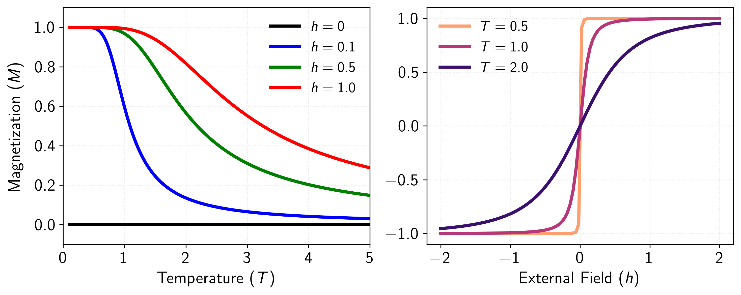
1. Magnetization $m(T,h)$:

   • For any finite temperature ($T>0$), if we set the external field to zero ($h=0$), the numerator $\sinh (0)=0$, so the magnetization $m(T,0)=0$. This confirms our earlier finding: there is no spontaneous magnetization at any non-zero temperature. The system cannot sustain long-range order on its own.
   • At zero temperature ($T=0⟹\beta \to \infty$), the term $e^{-4\beta J}$ goes to zero. The expression simplifies to $m(0,h)=\frac{\sinh (\beta h)}{|\sinh (\beta h)|}=\text{sgn}(h)$. The magnetization jumps discontinuously from -1 to +1 as the field crosses zero. The system is perfectly ordered, and an infinitesimal field is enough to align all spins. This is a phase transition, but it occurs only at the absolute zero of temperature.
   • The plot on the right shows that for any $T>0$, the curve $m(h)$ is smooth and continuous through $h=0$, becoming progressively steeper as $T$ decreases.

2. Susceptibility $\chi (T)$:

   • The susceptibility $\chi (T)$ is finite for any temperature $T>0$. A divergence in susceptibility often signals an impending phase transition, as it implies an infinite response to an infinitesimal field. The absence of such a divergence for $T>0$ is another definitive piece of evidence against a finite-temperature phase transition.
   • As $T\to 0$, the exponential term $e^{2J/k_{B}T}$ causes the susceptibility to diverge exponentially. This indicates that as the system approaches absolute zero, it becomes extremely sensitive to an external field, which is consistent with the onset of perfect order at $T=0$.

Conclusion

In this lesson, we have completed the exact solution of the 1D Ising model by extending the transfer matrix method to include an external magnetic field. By calculating the eigenvalues of the generalized transfer matrix, we obtained the exact free energy as a function of both temperature and field.

Key Takeaways:

• The transfer matrix for the 1D Ising model in a field $h$ is given by $T=\left(\begin{array}{cc}{e}^{\beta (J+h)}& e^{-\beta J}\\ e^{-\beta J}& e^{\beta (J-h)}\end{array}\right)$.
• The free energy per spin is determined by the largest eigenvalue, $f(T,h)=-k_{B}T\ln ({\lambda }_{+})$, and is analytic for all $T>0$ and any finite $h$.
• The exact magnetization is $m(T,h)=\sinh (\beta h)/\sqrt{{\sinh }^2(\beta h)+e^{-4\beta J}}$. This shows $m=0$ for $h=0$ and $T>0$, proving the absence of spontaneous magnetization.
• The zero-field susceptibility, $\chi (T)=\frac{1}{k_{B}T}{e}^{2J/k_{B}T}$, diverges exponentially as $T\to 0$ but is finite for any $T>0$, confirming the absence of a finite-temperature phase transition.

We now have a complete picture not only of the model's equilibrium state but also its response to external fields. However, the free energy and its derivatives only tell part of the story. They are macroscopic quantities. To gain a deeper, microscopic understanding of the order within the system, we need to investigate how the state of one spin is related to the state of another some distance away. In our next lesson, we will do just that by using the transfer matrix formalism to compute the spin-spin correlation function and the correlation length, which quantitatively describes the scale over which order persists in the system.