Spin-Spin Correlation in the 1D Ising Model

Introduction

In our last lesson, we finalized the exact solution of the 1D Ising model by incorporating an external magnetic field. Using the transfer matrix method, we derived the free energy, magnetization, and susceptibility, confirming that the model exhibits no spontaneous magnetization or phase transition at any finite temperature ( $T > 0$ ). These macroscopic observables, while crucial, average over the entire system and don't fully reveal the microscopic nature of its internal order.

Today, we will delve deeper into the microscopic structure by exploring how order decays with distance. Our objective is to define the spin-spin correlation function and compute the correlation length for the 1D Ising model. This will allow us to quantify precisely how the orientation of a single spin influences its neighbors, both near and far. By applying the powerful transfer matrix formalism once more, we will see that correlations decay exponentially, and the characteristic scale of this decay—the correlation length—provides the most definitive evidence yet for why long-range order cannot be sustained in one dimension at finite temperature.

1. The Concept of Correlation

At the heart of cooperative phenomena is the idea that the state of one particle is not independent of its neighbors. We need a mathematical tool to describe this interdependence. This tool is the spin-spin correlation function, typically defined for two spins at sites $i$ and $j$ as the thermal average of their product:

G (r) = ⟨ σ_{i} σ_{j} ⟩ where r = ∣ i - j ∣

Often, we use the connected correlation function, $G_{c} (r) = ⟨ σ_{i} σ_{j} ⟩ - ⟨ σ_{i} ⟩ ⟨ σ_{j} ⟩$ , which subtracts the trivial correlation arising from any background magnetization. For the 1D Ising model in zero field, the average magnetization $⟨ σ_{i} ⟩$ is zero by symmetry for any $T > 0$ , so the two functions are identical, $G (r) = G_{c} (r)$ .

What does $G (r)$ tell us?

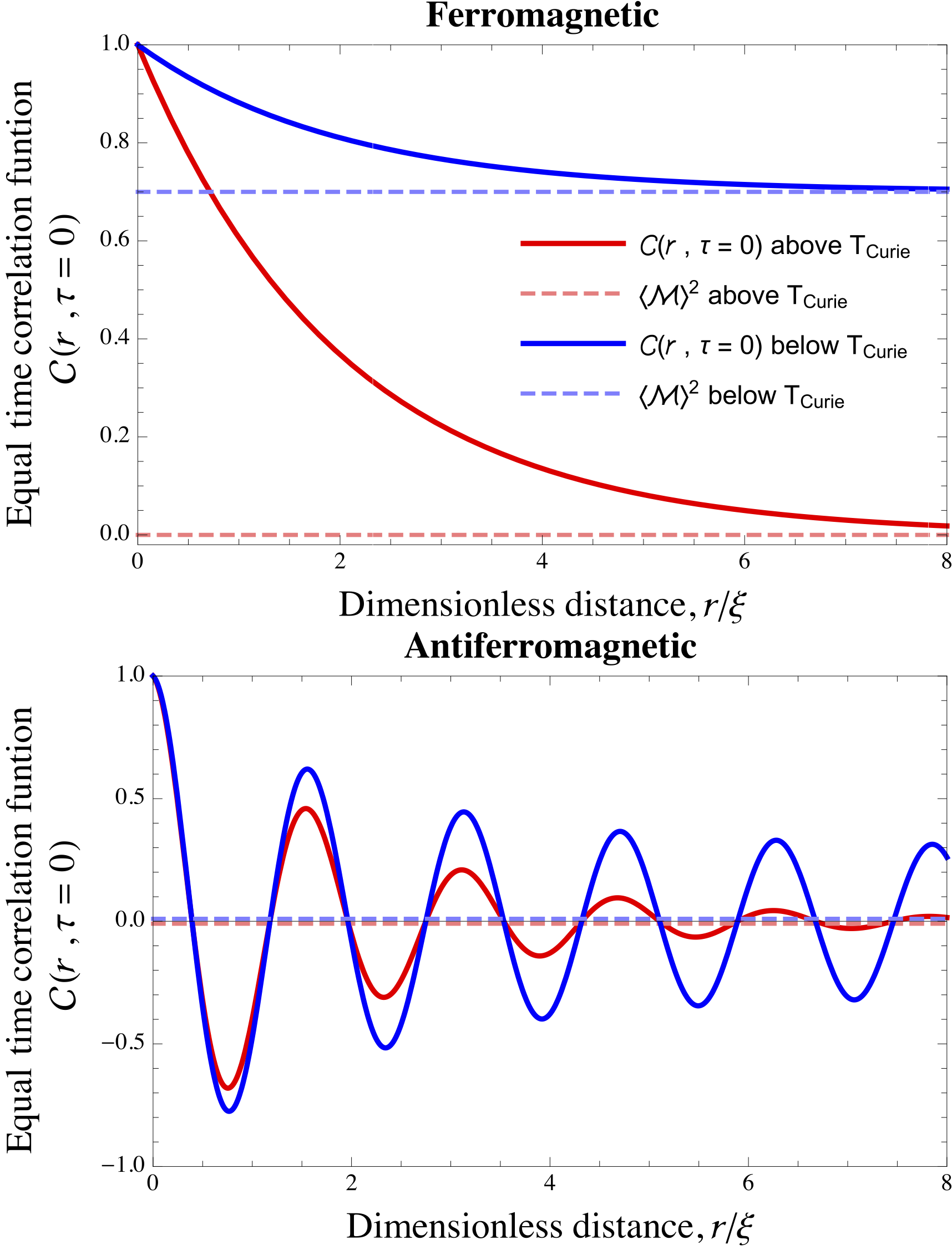
If spins become completely uncorrelated at large distances, we expect $G (r) \to ⟨ σ_{i} ⟩ ⟨ σ_{j} ⟩ = 0$ as $r \to \infty$ .
If a system exhibits long-range order, knowing the orientation of a spin far away gives us information about the spin at our location. In this case, $G (r)$ would approach a non-zero constant as $r \to \infty$ .

Before diving into the calculation, it's helpful to build some intuition for what we expect. Professor Susskind offers a wonderful analogy.

Statistical Mechanics Lecture 9

In this excerpt from his Statistical Mechanics lecture, Leonard Susskind introduces the idea of the correlation function and provides a compelling analogy to understand why correlations must decay in a one-dimensional system.

First, watch the section from "I would like to know" where he poses the central question: how does knowing one spin's orientation affect another's far down the chain? Then, continue watching as he develops the "game of telephone" analogy. This vividly illustrates how small, local "errors" (thermal fluctuations) accumulate over distance, inevitably destroying any long-range message (correlation).

Susskind's analogy suggests that at any finite temperature (imperfect fidelity), the correlation must decay with distance. Our task now is to make this quantitative using the transfer matrix.

2. Correlation Function from the Transfer Matrix

Recall from the previous lesson that the partition function for a chain with periodic boundary conditions is $Z_{N} = Tr (T^{N})$ . To calculate the thermal average of a quantity like $σ_{i} σ_{j}$ , we must insert these operators into the sum over states that defines the partition function.

The key insight is that the spin variable $σ_{k}$ at a specific site $k$ can be represented by the Pauli matrix $σ^_{z} = (10 0 - 1)$ acting on the vector space of that site's spin states. When we write the partition function as a product of transfer matrices, inserting $σ_{k}$ is equivalent to inserting $σ^_{z}$ into the matrix product at the appropriate position.

This leads to the following expression for the correlation function between spins separated by $r$ sites on a ring of $N$ sites:

⟨ σ_{i} σ_{i + r} ⟩ = \frac{1}{Z _{N}} {σ} \sum σ_{i} σ_{i + r} k = 1 \prod N e^{β J σ_{k} σ_{k + 1}} = \frac{1}{Z _{N}} Tr (T^{N - r} σ^_{z} T^{r} σ^_{z})

This formula is the starting point for our calculation. The following reading from an MIT OCW problem set provides a concise and elegant derivation of the result.

[PDF] Statistical Mechanics II: Problem Set 4: Transfer Matrices & Position ...

This problem set provides a direct calculation of the two-spin correlation function for the 1D Ising model in zero field.

Start reading from the paragraph that begins "A more interesting quantity" (p. 2). This section sets up the trace expression for \langle \sigma_i \sigma_{i+r} \rangle and evaluates it by rotating to the basis where the transfer matrix T is diagonal. Focus on how the trace simplifies in this basis.

To carry out the calculation, we need the eigenvalues and eigenvectors of the zero-field transfer matrix:

T = (e^{β J} e^{- β J} e^{- β J} e^{β J})

As you know from our first lesson on this topic, the eigenvalues are $λ_{+} = 2 cosh (β J)$ and $λ_{-} = 2 sinh (β J)$ . The corresponding eigenvectors are $v_{+} = \frac{1}{2} (11)$ and $v_{-} = \frac{1}{2} (1 - 1)$ .

The calculation in the reading shows that, after transforming to the basis of these eigenvectors and taking the thermodynamic limit $N ≫ r$ , the correlation function simplifies dramatically:

⟨ σ_{i} σ_{i + r} ⟩ = (\frac{λ _{-}}{λ _{+}})^{r} = (\frac{2 sinh ( β J )}{2 cosh ( β J )})^{r} = (tanh (β J))^{r}

This is a beautiful and compact result. It confirms the "game of telephone" intuition: the correlation decays geometrically (exponentially) with distance $r$ . The "fidelity" of transmission from one site to the next is given by $tanh (β J)$ .

3. The Correlation Length

The standard form for an exponentially decaying correlation function is $G (r) \sim e^{- r / ξ}$ , where $ξ$ is the correlation length. It represents the characteristic length scale over which the spins are significantly correlated.

Comparing our result to this standard form, we have:

(tanh (β J))^{r} = (e^{l n (t a n h (β J))})^{r} = e^{r l n (t a n h (β J))} = e^{- r / ξ}

From this, we can immediately identify the correlation length:

ξ = - \frac{1}{ln ( tanh ( β J ))}

Let's examine the behavior of $ξ$ in different temperature regimes.

[PDF] Lecture Notes

These notes formalize the definition of the correlation length and analyze its asymptotic behavior.

Please read the section starting from "Now, consider the model" (p. 2). This part provides the explicit formula for \xi in the zero-field case and examines its behavior as T \to 0.

As shown in the notes, the behavior of the correlation length is very telling:

High Temperature ( $T \to \infty$ , $β \to 0$ ):
$tanh (β J) \approx β J$ . Since $β J ≪ 1$ , $ln (β J)$ is large and negative, so $ξ = - 1/ ln (β J) \to 0$ . The spins are essentially uncorrelated beyond their immediate neighbors. The system is a disordered paramagnet.
Low Temperature ( $T \to 0$ , $β \to \infty$ ):
Using the approximation $tanh (x) \approx 1 - 2 e^{- 2 x}$ for large $x$ , we get $tanh (β J) \approx 1 - 2 e^{- 2 β J}$ . Then, using $ln (1 - y) \approx - y$ for small $y$ , we find $ln (tanh (β J)) \approx - 2 e^{- 2 β J}$ .
This gives a correlation length of:
$ξ \approx \frac{1}{2} e^{2 β J} = \frac{1}{2} e^{2 J / k_{B} T}$
The correlation length diverges exponentially as the temperature approaches absolute zero. This means that at very low temperatures, large domains of aligned spins can form. However, $ξ$ remains finite for any $T > 0$ , only becoming infinite at the critical point $T_{c} = 0$ .

The divergence of the correlation length is the hallmark of a continuous phase transition. The fact that $ξ$ only diverges at $T = 0$ is the most fundamental reason why the 1D Ising model is not ordered at any finite temperature.

A visualization of the 1D Ising model on a ring, with spins $S_i = \pm 1$. The correlation function $\langle S_i S_{i+r} \rangle$ measures the tendency for spins separated by $r$ sites to align.

4. A Physical Picture: Domain Walls

While the transfer matrix calculation is exact and powerful, there is a more intuitive physical argument that reproduces the low-temperature behavior of $ξ$ . Given your work with bubble rafts and avalanches, you may find this picture of excitations and "defects" particularly appealing.

Consider the ground state at $T = 0$ : all spins are aligned, either all up or all down. The lowest-energy excitation is to flip a semi-infinite chain of spins, creating a single "domain wall"—a boundary between a region of up spins and a region of down spins. This frustrates exactly one bond, costing an energy of $Δ E = J - (- J) = 2 J$ .

At a low but finite temperature $T$ , these domain walls can be thermally excited. The probability of finding a domain wall at any given bond is suppressed by a Boltzmann factor, $p \sim e^{- Δ E / k_{B} T} = e^{- 2 β J}$ .

If these domain walls are rare (which they are at low $T$ ), we can think of them as a dilute gas of defects. The average distance between these defects is simply the inverse of their density, $1/ p$ . This average distance is precisely the scale over which a domain of aligned spins can persist before being interrupted. Therefore, we can identify the correlation length with this average distance:

ξ \sim \frac{1}{p} \sim e^{2 β J}

This beautifully simple argument reproduces the exponential divergence we found from the rigorous transfer matrix calculation. It provides a powerful physical intuition: the correlation length is determined by the density of thermally excited defects that break the local order.

Spatial correlation functions for ferromagnetic (top) and antiferromagnetic (bottom) systems. Our result for the 1D Ising model, $G(r) = (\tanh(\beta J))^r$, corresponds to the ferromagnetic case. Note how correlations decay to zero over a distance of a few correlation lengths ($r/\xi$), but this decay becomes slower (i.e., $\xi$ grows) as the system is cooled toward its critical temperature.

Conclusion

In this lesson, we have moved from macroscopic thermodynamics to the microscopic structure of order in the 1D Ising model. By defining and calculating the spin-spin correlation function, we have developed a quantitative measure for the range of spin alignment.

Key Takeaways:

The spin-spin correlation function $⟨ σ_{i} σ_{i + r} ⟩$ quantifies the influence of a spin's orientation on another spin at a distance $r$ .
Using the transfer matrix formalism, we found the exact result for the 1D Ising model in zero field: $⟨ σ_{i} σ_{i + r} ⟩ = (tanh (β J))^{r}$ . This shows that correlations decay exponentially with distance.
The characteristic scale of this decay is the correlation length, $ξ = - 1/ ln (tanh (β J))$ .
The correlation length $ξ$ is finite for any $T > 0$ and diverges exponentially only as $T \to 0$ . This confirms the absence of a finite-temperature phase transition, as such a transition requires the correlation length to diverge at a non-zero critical temperature $T_{c}$ .
Physically, the correlation length at low temperatures can be understood as the average distance between thermally excited domain walls.

Having exhaustively analyzed the 1D Ising model and understood why it fails to order, we are now equipped to study the richer phenomena of phase transitions in higher dimensions. In the next lesson, we will begin building a general phenomenological framework by classifying phase transitions and defining the concepts of order parameters and critical exponents, which are essential for describing the universal behavior of systems near a critical point.

Recommended resources