Mean-Field Approximation for the Ising Model

In our previous lesson, we established the Ising model as a fundamental paradigm for understanding interacting systems and the cooperative phenomena they exhibit, like phase transitions. We saw that the interaction term, $- J \sum_{⟨ i, j ⟩} s_{i} s_{j}$ , couples all the spins together, making an exact solution for the system's partition function intractable in most cases.

Today, we will develop our first and most important tool for analyzing such systems: Mean-Field Theory (MFT). The goal of this lesson is to derive the mean-field (or Bragg-Williams) approximation for the Ising model by neglecting fluctuations. This powerful approximation reduces the complex, interacting many-body problem to a much simpler, solvable single-body problem, allowing us to gain our first quantitative insights into the nature of phase transitions. We will explore this approximation from two complementary perspectives: an intuitive physical argument and a more formal variational approach.

1. The Core Idea: Replacing Neighbors with an Average

The difficulty in the Ising model lies in the fact that the state of a spin $s_{i}$ is correlated with the state of its neighbor $s_{j}$ , which in turn is correlated with its neighbors, and so on, creating a complex web of dependencies across the entire lattice. The central idea of mean-field theory is to sever this web by making a radical simplification: we assume that each spin does not feel the instantaneous state of its individual neighbors, but rather feels an average, or mean, field generated by all of them.

This video from the channel Pretty Much Physics provides a clear overview of the general strategy behind any mean-field theory.

Mean-Field Theory | Ising model | Solid State Physics

This video outlines the three general steps of MFT and then applies them to the Ising model, focusing on the key approximation step.

Watch the introduction which lays out the three core steps of any mean-field theory. Next, watch the segment that re-introduces the Ising Hamiltonian and explains the key approximation: neglecting correlation effects. Pay close attention to how the interaction term is re-written.

The key step, as shown in the video, is to handle the problematic interaction term $s_{i} s_{j}$ . The approximation hinges on the idea of neglecting fluctuations. Let's make this more precise. We can write any spin variable $s_{i}$ as the sum of its thermal average $⟨ s_{i} ⟩$ and a fluctuation $δ s_{i}$ around that average:

s_{i} = ⟨ s_{i} ⟩ + δ s_{i}

The interaction term between two neighboring spins then becomes:

s_{i} s_{j} = (⟨ s_{i} ⟩ + δ s_{i}) (⟨ s_{j} ⟩ + δ s_{j}) = ⟨ s_{i} ⟩ ⟨ s_{j} ⟩ + ⟨ s_{i} ⟩ δ s_{j} + ⟨ s_{j} ⟩ δ s_{i} + δ s_{i} δ s_{j}

Mean-field theory consists of neglecting the term that is second-order in the fluctuations, $δ s_{i} δ s_{j}$ . This is the mathematical embodiment of "neglecting correlations". Assuming translational invariance, the average value of any spin is the same, which we define as the magnetization per site, $m = ⟨ s_{i} ⟩$ . The approximation for the interaction term then simplifies to:

s_{i} s_{j} \approx m^{2} + m (s_{j} - m) + m (s_{i} - m) = m (s_{i} + s_{j}) - m^{2}

This algebraic manipulation is the heart of the approximation. Let's see how it transforms the full Hamiltonian.

2. The Mean-Field Hamiltonian

We start with the Ising Hamiltonian:

H = - J ⟨ i, j ⟩ \sum s_{i} s_{j} - h i \sum s_{i}

Now, we substitute our approximation for the interaction term $s_{i} s_{j}$ :

H \approx - J ⟨ i, j ⟩ \sum [m (s_{i} + s_{j}) - m^{2}] - h i \sum s_{i}

Let's analyze the sum $\sum_{⟨ i, j ⟩}$ . It runs over all unique nearest-neighbor pairs. If the lattice has $N$ sites and each site has $q$ nearest neighbors (the coordination number), the total number of bonds is $q N /2$ . Therefore, $\sum_{⟨ i, j ⟩} m^{2} = \frac{q N}{2} m^{2}$ .

The sum $\sum_{⟨ i, j ⟩} (s_{i} + s_{j})$ can be rewritten. Each spin $s_{k}$ is a member of $q$ different pairs. So, when we sum over all pairs, each $s_{k}$ appears $q$ times. Thus, $\sum_{⟨ i, j ⟩} (s_{i} + s_{j}) = q \sum_{i} s_{i}$ .

Substituting these back into the Hamiltonian gives:

H_{MF} = - J (q i \sum m s_{i} - \frac{q N}{2} m^{2}) - h i \sum s_{i}

Rearranging terms, we get:

H_{MF} = - (J q m + h) i \sum s_{i} + \frac{N q J}{2} m^{2}

This is the Mean-Field Hamiltonian. Notice its structure. The second term is just a constant energy offset that depends on the (yet unknown) average magnetization $m$ . The first term looks exactly like the Hamiltonian for $N$ non-interacting spins in an effective magnetic field $h_{eff} = J q m + h$ .

We have successfully reduced the interacting problem to a non-interacting one. The price we paid is that the effective field now depends on the average magnetization $m$ , which is the very quantity we want to calculate. This leads to a self-consistency condition.

The following video provides an excellent walkthrough of this derivation.

Lecture 42: Mean Field Theory

This lecture from NPTEL IIT Kharagpur provides a clear, step-by-step derivation of the mean-field approximation and the resulting self-consistency equation.

Begin by watching the introduction to the MFT approximation, which emphasizes the neglect of thermal fluctuations. Next, follow the crucial algebraic derivation from approximating the s_i s_j term. This directly corresponds to the steps we just outlined. Finally, see how this leads to the concept of an effective field and the self-consistency equation.

As derived in the video and from our analysis, the average magnetization of a single spin in the effective field $h_{eff}$ is given by the well-known result for a paramagnet:

m = tanh (β h_{eff}) = tanh (β (J q m + h))

This is the central result of mean-field theory: a self-consistency equation for the magnetization $m$ .

3. The Bragg-Williams Approximation: A Variational Approach

The derivation above is physically intuitive. A more formal and powerful method, which you will appreciate given your mathematical background, is the variational approach based on the Gibbs-Bogoliubov inequality. This inequality states that for a system with a true Hamiltonian $H$ , the true free energy $F$ is bounded from above by a variational free energy $F_{V}$ constructed from a simpler, solvable "trial" Hamiltonian $H_{0}$ :

F \leq F_{0} + ⟨ H - H_{0} ⟩_{0} \equiv F_{V}

Here, $F_{0}$ is the free energy of the trial system, and the average $⟨ \dots ⟩_{0}$ is a thermal average taken with respect to the Boltzmann distribution of $H_{0}$ . The best approximation to $F$ is found by choosing $H_{0}$ such that $F_{V}$ is minimized.

For the Ising model, we choose a non-interacting trial Hamiltonian with a variational parameter $λ$ (which will play the role of an effective field):

H_{0} = - λ i \sum s_{i}

The key physical assumption of the Bragg-Williams approximation is that the spins are uncorrelated. This is automatically satisfied by our choice of a non-interacting $H_{0}$ . The derivation involves calculating the terms in $F_{V}$ and minimizing with respect to $λ$ .

The following paper provides a detailed, rigorous derivation using this variational method. It is an excellent example of the formal underpinnings of MFT.

MAGNETISATION AND MEAN FIELD THEORY IN THE ISING MODEL

This article provides a rigorous, step-by-step derivation of the mean-field model using variational methods, perfect for appreciating the mathematical structure of the approximation.

Please read the entire subsection Deriving a mean field model. The author uses m for the variational field parameter where we used \lambda. Follow the calculation of the variational free energy F_V and its minimization. Note specifically how the assumption of uncorrelated spins (\langle s_i s_j \rangle_0 = \langle s_i \rangle_0 \langle s_j \rangle_0) is used to simplify the expectation value term.

As you have worked through in the reading, the minimization of the variational free energy, $\partial F_{V} / \partial λ = 0$ , leads to an optimal value for the variational field $λ = J q m + h$ , where $m = tanh (β λ)$ . Substituting $λ$ back gives us precisely the same self-consistency equation we found earlier:

m = tanh (β (J q m + h))

This confirms that the intuitive physical picture of replacing neighbors with their average is equivalent to the more formal Bragg-Williams variational approach, which assumes a factorized (uncorrelated) probability distribution for the spins.

4. Graphical Solution and Spontaneous Magnetization

Let's examine the self-consistency equation in the absence of an external field ( $h = 0$ ):

m = tanh (β J q m)

This is a transcendental equation for $m$ , which can be solved graphically by plotting $y_{1} = m$ and $y_{2} = tanh (β J q m)$ and finding their intersections.

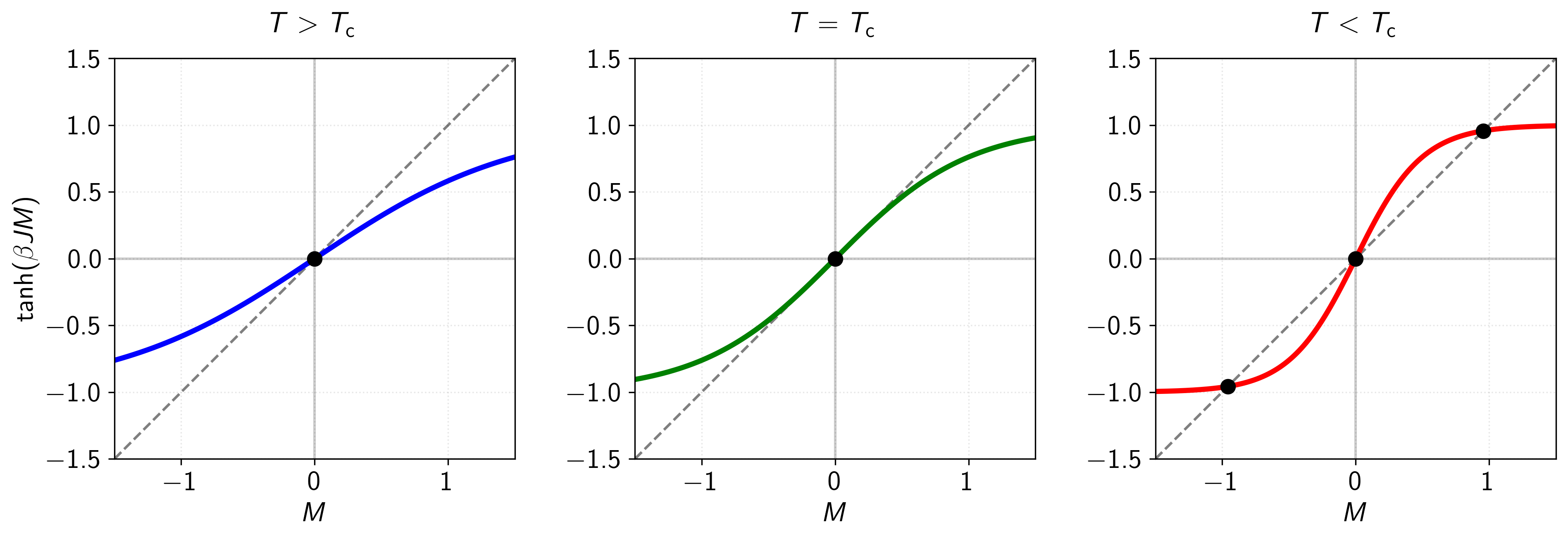
Solutions to the mean-field equation $m = \tanh(\beta Jq m)$. The intersections of the straight line $y=m$ and the curve $y=\tanh(\beta Jq m)$ give the possible values for the magnetization. The behavior depends critically on the temperature $T$, which enters through $\beta = 1/k_B T$.

Let's analyze the graphs:

High Temperature ( $T > T_{c}$ ): Here, $β$ is small. The initial slope of $tanh (x)$ at $x = 0$ is 1. The slope of $y_{2}$ at the origin is $β J q$ . When $T$ is high, $β J q < 1$ , so the slope of the tanh curve is less than the slope of the line $y_{1} = m$ . The only intersection is at $m = 0$ . There is no spontaneous magnetization; the system is in a disordered paramagnetic state.
Low Temperature ( $T < T_{c}$ ): Here, $β$ is large, and the initial slope $β J q > 1$ . The tanh curve is steeper than the line $y_{1} = m$ at the origin. This results in three intersections: one at $m = 0$ (which turns out to be an unstable solution) and two symmetric solutions at $m = \pm m_{0}$ . The system spontaneously chooses one of these states, breaking the up/down symmetry and developing a non-zero magnetization $m_{0} \neq = 0$ . This is the ordered ferromagnetic state.
Critical Temperature ( $T = T_{c}$ ): The transition occurs exactly when the initial slope of the tanh curve equals the slope of the line $y = m$ . This condition is $β_{c} J q = 1$ . This allows us to determine the critical temperature in mean-field theory: $k_{B} T_{c} = J q$

Conclusion

In this lesson, we have derived the mean-field approximation for the Ising model, our first analytical tool for studying an interacting system. We have seen that this powerful approximation, which simplifies the problem by neglecting correlations between spin fluctuations, can be reached through both an intuitive physical argument and a more formal variational principle.

Key Takeaways:

Mean-field theory replaces the instantaneous interaction of a spin with its neighbors with an interaction with an average or "mean" field generated by them.
This is equivalent to assuming spins are uncorrelated, i.e., $⟨ s_{i} s_{j} ⟩ \approx ⟨ s_{i} ⟩ ⟨ s_{j} ⟩$ , which means neglecting the correlation of fluctuations.
The approximation reduces the interacting many-body problem to a solvable single-body problem in an effective magnetic field, $h_{eff} = J q m + h$ .
This leads to a self-consistency equation for the magnetization: $m = tanh (β (J q m + h))$ .
The Bragg-Williams approximation provides a formal justification for this via the Gibbs-Bogoliubov variational principle, where the mean-field free energy is the best possible upper bound achievable with a non-interacting trial Hamiltonian.

We have derived the central equation of MFT and used it to identify the existence of a phase transition. In the next lesson, we will analyze this equation in more detail. We will solve it near the critical point to calculate the critical exponents $β$ , $γ$ , and $δ$ , which characterize the singular behavior of physical quantities at the phase transition.

Recommended resources

1. The Core Idea: Replacing Neighbors with an Average

2. The Mean-Field Hamiltonian

3. The Bragg-Williams Approximation: A Variational Approach

4. Graphical Solution and Spontaneous Magnetization

Conclusion