Mean-Field Magnetization and Critical Temperature

1. Graphical Solution and the Critical Temperature

Let's begin with the simplest case: zero external magnetic field ($h=0$). The self-consistency equation becomes:

This is a transcendental equation, meaning it cannot be solved for $m$ algebraically. However, we can gain significant insight by solving it graphically. The solutions are the points of intersection between the two functions:

1. $y_1(m)=m$ (a straight line with slope 1)
2. $y_2(m)=\tanh (ax)$ where $a=\beta Jq$ and the variable is $m$.

The shape of the hyperbolic tangent curve, and thus the number of solutions, depends critically on its initial slope at $m=0$. The derivative of $\tanh (am)$ with respect to $m$ is $a\cdot {\mathrm{sech}}^2(am)$. At $m=0$, this slope is simply $a=\beta Jq=\frac{Jq}{k_{B}T}$. The behavior of the system falls into three distinct regimes depending on temperature.

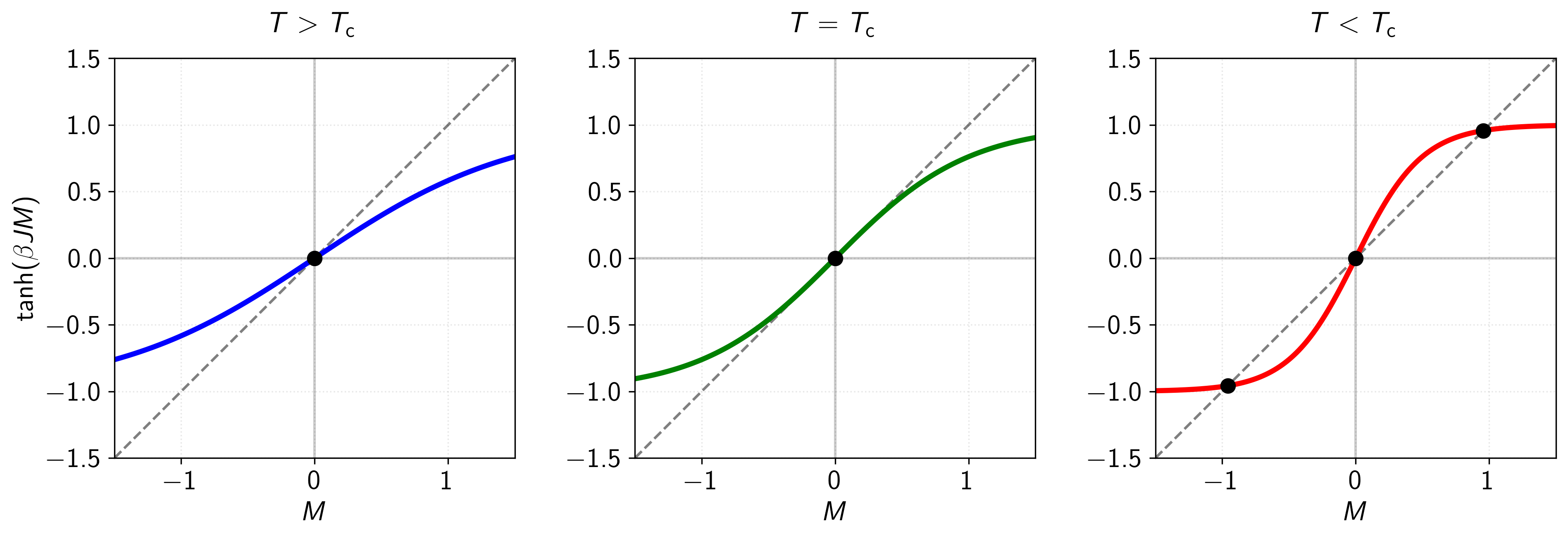
Let's analyze the three cases shown in the image:

• High Temperature ($T>T_c$): When the temperature is high, $\beta$ is small, so the initial slope $\beta Jq<1$. The $\tanh$ curve (blue) is less steep than the line $y=m$. The only intersection is at $m=0$. This means there is no spontaneous magnetization, and the system is in a disordered paramagnetic state.

• Low Temperature ($T<T_c$): At low temperatures, $\beta$ is large, and the initial slope $\beta Jq>1$. The $\tanh$ curve (red) is steeper than $y=m$ at the origin. This leads to three intersection points: one at $m=0$ and two symmetric solutions at $m=\pm m_0$. As we will see when we consider the free energy, the $m=0$ solution is unstable, while the two non-zero solutions $m=\pm m_0$ are the stable, equilibrium states. The system spontaneously picks one of these states, breaking the $m\to -m$ symmetry and developing a non-zero magnetization. This is the ordered ferromagnetic state.

• Critical Temperature ($T=T_c$): The transition between these two regimes occurs at the precise temperature where the initial slope of the $\tanh$ curve is exactly equal to the slope of the line $y=m$. This critical condition is:

  $${\beta }_{c}Jq=1$$

  Substituting ${\beta }_c=1/(k_B{T}_c)$, we can solve for the mean-field critical temperature:

  $$k_B{T}_c=Jq$$

  Here, $q$ is the coordination number of the lattice. This is a central prediction of mean-field theory: the transition temperature is proportional to the interaction strength $J$ and the number of interacting neighbors $q$.

The following reading from Daniel Arovas's lecture notes provides a clear and concise derivation of these results.

2. Analytical Solution Near $T_c$

The graphical method is illustrative, but to find the functional form of $m(T)$ just below the critical temperature, we need an analytical approach. As we approach $T_c$ from below, the magnetization $m$ becomes very small. This allows us to Taylor expand the $\tanh$ function in the self-consistency equation: $\tanh (x)\approx x-x^3/3+\dots$

Let $x=\beta Jqm$. The equation $m=\tanh (x)$ becomes:

We are interested in the non-trivial solution $m\ne 0$, so we can divide the equation by $m$:

Recalling that $k_B{T}_c=Jq$, we can write $\beta Jq=\frac{Jq}{k_{B}T}=\frac{T_c}{T}$. Substituting this in gives:

Rearranging to solve for $m^2$:

For temperatures just below the critical point, $T\approx T_c$, so we can approximate $T/T_c^2\approx T_c/T_c^2=1/T_c$. This yields the characteristic behavior of the order parameter near the critical point:

This tells us that the spontaneous magnetization vanishes continuously as $T$ approaches $T_c$ from below, with a characteristic power-law behavior. The exponent, in this case 1/2, is a "critical exponent" which we will study systematically in the next lesson.

3. The Role of an External Field

Now let's return to the full self-consistency equation, including an external field $h$:

The presence of the field $h$ breaks the up/down ($m\to -m$) symmetry of the system.

• For $T<T_c$, a positive field $h>0$ favors the $+m_0$ solution, making it the unique ground state.
• For $T>T_c$, where the spontaneous magnetization is zero, the field induces a non-zero magnetization, as expected for a paramagnet.

Let's investigate the paramagnetic response for $T>T_c$ where $h$ is small. Since $h$ is small, the induced magnetization $m$ will also be small. We can again linearize the $\tanh$ function: $\tanh (x)\approx x$.

Solving for $m$:

The isothermal magnetic susceptibility is defined as ${\chi }_T=(\frac{\partial m}{\partial h}{)}_{T,h\to 0}$. From our result, we find:

This is the celebrated Curie-Weiss law, which describes the susceptibility of a ferromagnet in its paramagnetic phase. Mean-field theory predicts that the susceptibility diverges as the temperature approaches the critical temperature from above, another hallmark of a continuous phase transition.

The following reading covers this derivation.

Conclusion

In this lesson, we have thoroughly analyzed the mean-field self-consistency equation, which has yielded our first quantitative picture of a phase transition. By solving this equation, we have uncovered the core phenomena associated with the ferromagnetic transition.

Key Takeaways:

• The self-consistency equation $m=\tanh (\beta Jqm)$ can be solved graphically, revealing three distinct temperature regimes.
• A critical temperature, $T_c$, separates a high-temperature paramagnetic phase ($m=0$) from a low-temperature ferromagnetic phase ($m\ne 0$).
• Mean-field theory predicts a specific value for the critical temperature: $k_B{T}_c=Jq$.
• For temperatures just below $T_c$, the spontaneous magnetization grows as $m(T)\propto (T_c-T{)}^{1/2}$.
• For temperatures above $T_c$, the magnetic susceptibility follows the Curie-Weiss law, ${\chi }_T\propto (T-T_c{)}^{-1}$, diverging at the critical point.

We have now seen how the magnetization and susceptibility behave near the critical point. In our next lesson, we will adopt a more powerful and general approach by analyzing the mean-field free energy. Expanding this free energy as a power series in the magnetization will allow us to systematically calculate the full set of critical exponents ($\beta ,\gamma ,\delta$, etc.) and gain a deeper thermodynamic understanding of the phase transition.