Critical Exponents from Mean-Field Free Energy

Hello! In our previous lesson, we derived and solved the mean-field self-consistency equation, giving us our first look at a continuous phase transition. We found the critical temperature $T_{c}$ and saw how the spontaneous magnetization $m$ and magnetic susceptibility $χ_{T}$ behave near this point, obtaining preliminary values for the exponents $β = 1/2$ and $γ = 1$ .

Today, we will formalize and generalize this analysis. Instead of working directly with the self-consistency equation, we will shift our focus to the mean-field free energy itself. By expanding this free energy in a power series of the magnetization—an approach that forms the foundation of the powerful Landau theory of phase transitions—we can systematically derive the critical exponents that characterize the singular behavior near $T_{c}$ . Our objective is to expand the mean-field free energy near $T_{c}$ to calculate the critical exponents $β$ , $γ$ , and $δ$ . This will provide a deeper thermodynamic perspective on the nature of the critical point.

1. The Landau Expansion of the Mean-Field Free Energy

Recall that the mean-field approximation leads to an effective free energy per spin, $f (m)$ , which depends on the average magnetization $m$ . This function's minimum with respect to $m$ gives the equilibrium state of the system. In the vicinity of a continuous phase transition, the order parameter (in this case, the magnetization $m$ ) is small. This crucial observation allows us to Taylor expand the free energy in powers of $m$ .

The general form of the mean-field free energy per spin is:

f (m, T, h) = (- \frac{1}{2} J q m^{2} - hm) - T S (m)

where the first term is the mean-field energy and $S (m)$ is the entropy associated with having an average magnetization $m$ . For a spin-1/2 system, this entropy term is $S (m) = - k_{B} [\frac{1 + m}{2} ln (\frac{1 + m}{2}) + \frac{1 - m}{2} ln (\frac{1 - m}{2})]$ .

Expanding this full expression for small $m$ and organizing by powers of $m$ yields what is known as the Landau free energy. For simplicity, we will set $k_{B} = 1$ from here on.

Statistical Field Theory

These notes from David Tong's lecture series on Statistical Field Theory provide a concise and elegant derivation of the Landau expansion.

First, briefly review the section "Mean Field Theory" to see how the free energy f(m) is constructed. Then, focus on the section "Landau Approach to Phase Transitions," particularly the derivation of the Taylor expansion of f(m) in equation (1.12). Please read from the beginning of Section 1.2 up to the expanded free energy expression. The result is: f(m) \approx -T \log 2 -hm + \frac{1}{2}(T -Jq)m^2 + \frac{T}{12}m^4 + \mathcal{O}(m^6) Notice how the coefficient of the m^2 term, (T-Jq), changes sign at the critical temperature T_c = Jq.

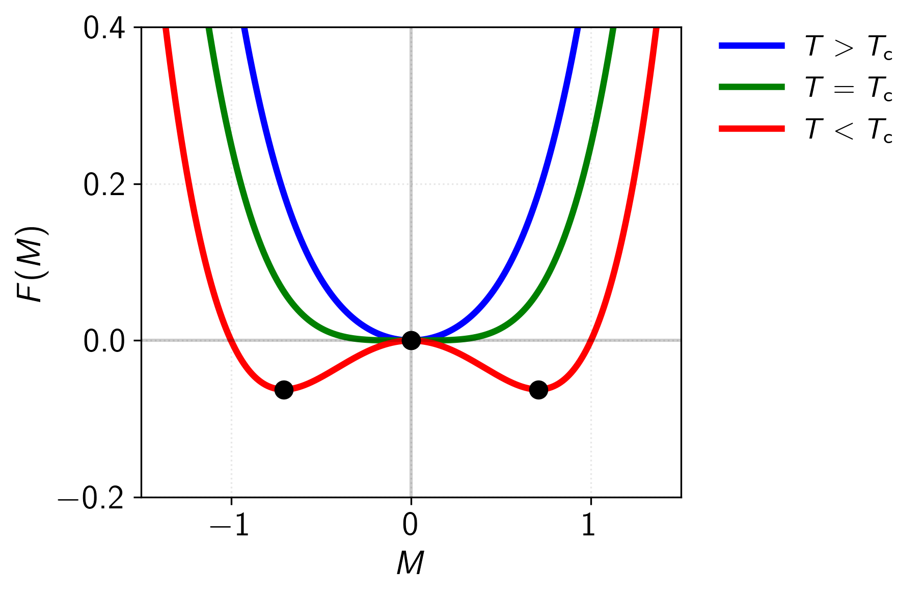
This expanded form, $f (m) \approx f_{0} - hm + a (T - T_{c}) m^{2} + b m^{4}$ , where $a$ and $b$ are positive constants, is the central tool for our analysis. The equilibrium magnetization is the value of $m$ that minimizes this function. The behavior of these minima as we vary temperature $T$ and external field $h$ dictates the physics of the phase transition.

The following video and figure provide excellent visual intuition for how the shape of this free energy landscape determines the phase of the system.

Landau Ginzburg theory of Phase Transitions

This video by Jos Thijssen introduces the Landau expansion and explains its key features.

Watch the segment from the introduction of the expansion. Pay attention to how the symmetry of the problem for h=0 dictates that only even powers of m appear, and how the sign of the quadratic coefficient, r_0 \propto (T-T_c), determines whether the system has one or two minima.

The Landau free energy $F(M)$ (equivalent to our $f(m)$) as a function of magnetization $M$ for different temperatures. Above $T_c$ (blue), there is a single minimum at $M=0$ (paramagnetic state). At $T_c$ (green), the curvature at the origin vanishes. Below $T_c$ (red), $M=0$ becomes an unstable maximum, and two new symmetric minima appear at non-zero magnetization (ferromagnetic state).

2. Calculation of Critical Exponents

The equilibrium state is found by minimizing the free energy with respect to the order parameter: $\frac{\partial f}{\partial m} = 0$ . Using the expanded form and ignoring the constant term, we get the equation of state:

\frac{\partial f}{\partial m} = - h + (T - T_{c}) m + \frac{T}{3} m^{3} \approx 0

We've approximated $T /3 \approx T_{c} /3$ in the $m^{3}$ term, as we are interested in the behavior near $T_{c}$ . This single equation contains all the information needed to find $β$ , $γ$ , and $δ$ .

The exponent $β$ : Spontaneous Magnetization

The exponent $β$ describes how the spontaneous magnetization $m_{0}$ grows as the temperature is lowered below $T_{c}$ in zero external field ( $h = 0$ ).

Set $h = 0$ in the equation of state: $(T - T_{c}) m + \frac{T _{c}}{3} m^{3} = 0$ .
This gives two solutions: the trivial one $m = 0$ , and $m (T - T_{c} + \frac{T _{c}}{3} m^{2}) = 0$ .
The non-trivial solution for the spontaneous magnetization $m_{0}$ is: $m_{0}^{2} = - 3 \frac{T - T _{c}}{T _{c}} = 3 \frac{T _{c} - T}{T _{c}}$
This real, non-zero solution exists only for $T < T_{c}$ . Taking the square root gives: $m_{0} (T) = \pm 3 (\frac{T _{c} - T}{T _{c}})^{1/2}$

By definition, $m_{0} \propto (T_{c} - T)^{β}$ . Comparing with our result, we find:

β = 1/2

The exponent $δ$ : Critical Isotherm

The exponent $δ$ characterizes the relationship between magnetization and field exactly at the critical temperature, $T = T_{c}$ .

Set $T = T_{c}$ in the equation of state. The linear term vanishes: $- h + \frac{T _{c}}{3} m^{3} = 0 ⟹ h = \frac{T _{c}}{3} m^{3}$
Inverting this relationship to find $m$ as a function of $h$ : $m (h) = (\frac{3}{T _{c}})^{1/3} h^{1/3}$

The critical exponent $δ$ is defined by $m \propto h^{1/ δ}$ at $T = T_{c}$ . We can immediately identify:

δ = 3

The exponent $γ$ : Magnetic Susceptibility

The exponent $γ$ describes the divergence of the isothermal magnetic susceptibility, $χ_{T} = (\frac{\partial m}{\partial h})_{T}$ , as $T \to T_{c}$ at zero field.
To find $χ_{T}$ , we can differentiate the equation of state with respect to $h$ at constant $T$ :

- 1 + (T - T_{c}) \frac{\partial m}{\partial h} + T_{c} m^{2} \frac{\partial m}{\partial h} = 0

Solving for $χ_{T} = \frac{\partial m}{\partial h}$ gives:

χ_{T} = \frac{1}{( T - T _{c} ) + T _{c} m ^{2}}

Now we must consider the approach to $T_{c}$ from above and below.

Above $T_{c}$ ( $T \to T_{c}^{+}$ ): In the paramagnetic phase, the spontaneous magnetization is $m = 0$ .
$χ_{T} = \frac{1}{T - T _{c}} \propto (T - T_{c})^{- 1}$
This is the Curie-Weiss law we found in the previous lesson.
Below $T_{c}$ ( $T \to T_{c}^{-}$ ): In the ferromagnetic phase, we substitute the expression for the spontaneous magnetization, $m_{0}^{2} = 3 (T_{c} - T) / T_{c}$ .
$χ_{T} = \frac{1}{( T - T _{c} ) + T _{c} ( 3 \frac{T _{c} - T}{T _{c}} )} = \frac{1}{- ( T _{c} - T ) + 3 ( T _{c} - T )} = \frac{1}{2 ( T _{c} - T )} \propto (T_{c} - T)^{- 1}$

In both cases, the susceptibility diverges as $∣ T - T_{c} ∣^{- 1}$ . The definition is $χ_{T} \propto ∣ T - T_{c} ∣^{- γ}$ , so we conclude:

γ = 1

Note that the amplitude of the divergence is twice as large above $T_{c}$ as it is below. Such universal amplitude ratios are another important feature of critical phenomena.

The following resources provide a complete walkthrough of these derivations.

1 Unit 4-4: Critical Exponents within the Mean-Field ...

This document provides a very direct, step-by-step calculation of the mean-field exponents by expanding the self-consistency equation itself, which is equivalent to minimizing the Landau free energy we've just discussed.

Read through the derivations for each exponent: The calculation for exponent δ. The calculation for exponent β. The calculation for exponent γ. This will solidify your understanding of the algebraic steps involved.

Landau Ginzburg theory of Phase Transitions

Returning to Thijssen's video, you can now see the explicit calculation of the exponents from the free energy minimization.

First, watch the derivation of exponent β. Then, the video briefly mentions the results for γ and δ, confirming the values we've just derived.

3. Summary and Validity

Let's collect our results. Mean-field theory, via the Landau expansion, predicts a set of critical exponents:

Exponent	Definition	Mean-Field Value
$β$	$m_{0} \propto (T_{c} - T)^{β}$ for $T < T_{c}, h = 0$	$1/2$
$δ$	$m \propto h^{1/ δ}$ for $T = T_{c}$	$3$
$γ$	$\chi_T \propto	T - T_c

These exponents are called "classical" or "mean-field" exponents. They are a universal prediction of any theory that neglects fluctuations in the way that mean-field theory does.

Left: Magnetization vs. Temperature for different external fields, illustrating the $m \propto (T_c-T)^{1/2}$ behavior for $h=0$ (black curve). Right: Magnetization vs. External Field for different temperatures. The curve for $T=T_c$ (if plotted) would exhibit the $m \propto h^{1/3}$ relation near $h=0$.

How accurate are these predictions? For the 2D Ising model, Onsager's exact solution gives $β = 1/8$ , $δ = 15$ , and $γ = 7/4$ . Clearly, the mean-field values are incorrect for $d = 2$ . The reason for this discrepancy is the core assumption of mean-field theory: the neglect of fluctuations. Near a critical point, fluctuations in the order parameter become strongly correlated over large distances, and they play a dominant role.

The Landau expansion is nonetheless a monumental achievement. It provides a universal framework for describing phase transitions based only on symmetry and the analyticity of the free energy. The failure of its predictions motivates the need for more advanced theories, like the renormalization group, which systematically account for the fluctuations that mean-field theory ignores. We will explore the range of validity of mean-field theory more formally when we derive the Ginzburg criterion in a future lesson.

Statistical Field Theory

This final reading summarizes the mean-field exponents and puts them in context by comparing them to exact and experimental results.

Please read the subsection titled "Critical Exponents". This table provides a stark comparison between the mean-field predictions and the true values for the Ising model in d=2 and d=3, highlighting the limitations we have discussed.

Conclusion

In this lesson, we have moved beyond the simple self-consistency equation to a more powerful analysis based on the Landau expansion of the mean-field free energy. This method not only streamlined the calculation of critical exponents but also introduced a general theoretical framework for studying phase transitions.

Key Takeaways:

Expanding the mean-field free energy near $T_{c}$ gives the Landau form: $f (m) \approx f_{0} - hm + a (T - T_{c}) m^{2} + b m^{4}$ .
The behavior of the system is determined by the minima of this polynomial, which change shape as the coefficient of the $m^{2}$ term passes through zero at $T_{c}$ .
Minimizing this free energy allows for a systematic calculation of the mean-field critical exponents:
- $β = 1/2$ (spontaneous magnetization)
- $δ = 3$ (critical isotherm)
- $γ = 1$ (susceptibility)
These "classical" exponents are a universal prediction of theories that neglect fluctuations, but they differ significantly from exact results in low dimensions, signaling the breakdown of the mean-field approximation near a critical point.

In our next lesson, we will continue our investigation of mean-field theories by examining another canonical model: the van der Waals equation of state for a liquid-gas system. We will see how it, too, can be understood as a mean-field theory and how it exhibits a similar critical point and set of exponents.

Recommended resources