Ergodic Hypothesis: Bridging Time and Ensemble Averages

1. Time Averages vs. Ensemble Averages

At the heart of the issue are two distinct ways of calculating the average value of a physical observable, say $f(\mathbf{x})$, where $\mathbf{x}$ is a microstate in phase space $\Gamma$.

The Time Average
This is the average value of $f$ measured for a single system as its state $\mathbf{x}(t)$ evolves over a long period. We start the system in a specific microstate ${\mathbf{x}}_0$ and track its trajectory. The time average, denoted $\overline{f}$, is formally defined as:

This is, in principle, the quantity an experimentalist measures by observing one system over a long time.

The Ensemble Average
This is the average value of $f$ over a collection (an ensemble) of identical systems at a single instant in time. We imagine preparing a vast number of systems, each in a different microstate, according to some probability distribution $\rho (\mathbf{x})$. The ensemble average, denoted $⟨f⟩$, is then:

If the ensemble represents an isolated system in equilibrium, we will soon see that $\rho (\mathbf{x})$ is uniform over the accessible region of phase space. This average is what theorists can often calculate using the methods of statistical mechanics.

The video below provides a clear conceptual introduction to these two types of averages.

The central question of statistical mechanics is: under what conditions can we assert that $\overline{f}=⟨f⟩$?

2. The Ergodic Hypothesis: Content and Justification

The ergodic hypothesis, in its modern form, states:

For an isolated system in equilibrium, the time average of any observable is equal to the ensemble average over the microcanonical ensemble, for almost all initial conditions.

The physical "content" of this hypothesis is the idea that a single system's trajectory, given enough time, will explore the entire accessible region of phase space. It doesn't just visit every region, but it does so in an "unbiased" way, spending an amount of time in any given region that is proportional to that region's phase-space volume.

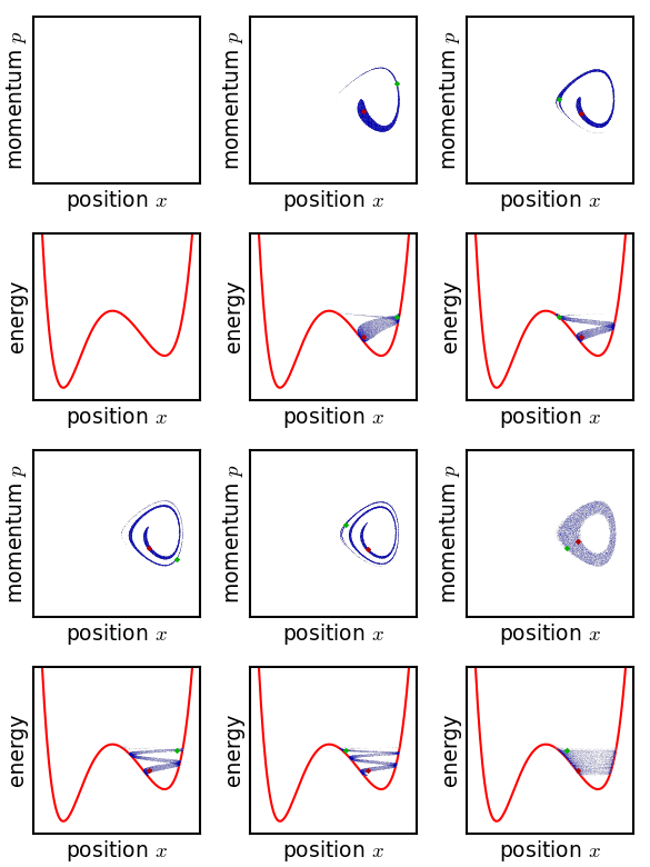
The GIF below animates a trajectory in a simple 2D phase space. For a particle with sufficient energy to overcome the central barrier, its trajectory explores a large portion of the available phase space, which is a necessary (though not sufficient) condition for ergodicity. If its energy were lower, confining it to one well, the system would clearly be non-ergodic with respect to the entire space, as it could never visit the other well.

Historically, the idea emerged from Boltzmann's work as a way to justify using probabilities in mechanics. The video segment below touches upon this historical context.

3. A More Rigorous View: Ergodicity and Invariant Sets

Your preference for mathematical rigor makes it worthwhile to delve deeper. Ergodic theory is a mature branch of mathematics that formalizes these ideas. Its foundational result is the Birkhoff Ergodic Theorem.

Birkhoff's Ergodic Theorem (1931): For any measure-preserving dynamical system (like a Hamiltonian system, thanks to Liouville's theorem) and any integrable function $f$, the time average $\overline{f}({\mathbf{x}}_0)$ exists for almost all initial points ${\mathbf{x}}_0$. Furthermore, the resulting limit function $\overline{f}({\mathbf{x}}_0)$ is itself an invariant of the motion, meaning $\overline{f}(\mathbf{x}(t))=\overline{f}({\mathbf{x}}_0)$ for all $t$.

This theorem guarantees that time averages exist, but it does not guarantee they are all the same value or that they equal the ensemble average. For that, we need the stronger condition of ergodicity. A system is ergodic if the only functions that are invariant along trajectories are constant functions (almost everywhere). If a system is ergodic, then $\overline{f}({\mathbf{x}}_0)$ must be a constant, independent of the initial state ${\mathbf{x}}_0$. It can then be shown that this constant must be equal to the ensemble average $⟨f⟩$.

The following resource provides a concise, mathematically rich overview of ergodicity, including several equivalent definitions that illuminate the concept from different angles.

The key takeaway is that ergodicity is the property that ensures a system's phase space cannot be decomposed into smaller, isolated sub-regions. The trajectory is forced to wander through the entire accessible volume, making its long-term average behavior representative of the whole.

4. Is Ergodicity True? Is It Necessary?

Proving that a realistic system of $10^{23}$ interacting particles is strictly ergodic is a task of formidable, and in most cases prohibitive, difficulty. While it has been proven for a few model systems (like a gas of hard spheres), it is widely believed that many realistic systems are not strictly ergodic.

Does this invalidate statistical mechanics? The modern answer is, surprisingly, no. The justification comes from a more subtle argument based on the concept of typicality, which you've encountered in your studies. For macroscopic systems, the equilibrium macrostate is "typical" in the sense that it corresponds to an overwhelmingly vast region of phase space.

A recent perspective, which you should find stimulating, argues that strict ergodicity is not a necessary assumption. Instead, a property called essential ergodicity emerges as a consequence for any system that has a stationary measure and a typical equilibrium state.

This powerful argument shifts the focus. We don't need to prove that every trajectory explores the phase space perfectly. We only need to show that the set of trajectories that don't behave this way is so vanishingly small that we would never expect to encounter one in a physical experiment. The sheer scale of macroscopic systems ensures that the system behaves as if it were ergodic.

Conclusion

In this lesson, we have confronted the foundational challenge of connecting single-system dynamics to ensemble theory. The ergodic hypothesis provides the conceptual and mathematical bridge.

Key Takeaways:

• The ergodic hypothesis posits the equality of the time average (measured on a single system over time) and the ensemble average (calculated over a collection of systems at one instant).
• The physical content of the hypothesis is that a single system's trajectory, over a long time, explores all accessible microstates in an unbiased manner, spending time in any region proportional to its phase-space volume.
• Mathematically, ergodicity is equivalent to the statement that a dynamical system has no non-trivial constants of motion besides energy, meaning its phase space cannot be decomposed into smaller invariant regions.
• While strict ergodicity is exceptionally difficult to prove and likely doesn't hold for many real systems, the modern view of essential ergodicity shows that the conclusion holds "for all practical purposes" (FAPP). This is a direct consequence of the fact that equilibrium macrostates occupy overwhelmingly large volumes of phase space.

This justification is the final conceptual step we need before we can confidently build the formal apparatus of statistical mechanics. In our next lesson, armed with the ergodic hypothesis, we will state the fundamental postulate of equal a priori probabilities and use it to formally define the microcanonical ensemble for an isolated system.