Liouville's Theorem: Phase-Space Incompressibility

In our previous lesson, we established the fundamental concepts of phase space, microstates, and macrostates, framing the arena for classical statistical mechanics. We saw that for a macroscopic system, a single macrostate corresponds to an immense number of microstates. However, we treated these as static snapshots. A real physical system is dynamic, its representative point continuously tracing a trajectory through phase space. Today, we will explore the rules governing the flow of an entire collection of such trajectories.

This leads us to one of the most elegant and foundational results in classical mechanics: Liouville's theorem. You will derive this theorem directly from Hamilton's equations and, crucially, interpret its physical meaning—the incompressibility of the phase-space "fluid." This theorem provides the mechanical basis for the principle of equal a priori probabilities, a cornerstone of statistical mechanics that we will encounter in a few lessons.

1. The Ensemble as a Fluid in Phase Space

Instead of focusing on a single system with one set of initial conditions, let's consider a conceptual collection of a vast number of identical systems, all governed by the same Hamiltonian but with slightly different initial conditions. This collection is called a statistical ensemble. Each system in the ensemble is represented by a single point in phase space. The entire ensemble, therefore, forms a cloud or "dust" of points in phase space.

As time evolves, each point follows its unique trajectory dictated by Hamilton's equations. The entire cloud of points flows through phase space, much like a fluid. We can define a "velocity field" for this imaginary fluid. At any point $x = (q_{1}, \dots, q_{3 N}, p_{1}, \dots, p_{3 N})$ in the $6 N$ -dimensional phase space, the velocity of the fluid, $x ˙$ , is simply the time derivative of the phase space coordinates:

x ˙ = (q ˙_{1}, \dots, q ˙_{3 N}, p ˙_{1}, \dots, p ˙_{3 N})

From your study of classical mechanics, you know that Hamilton's equations provide these velocities:

q ˙_{i} = \frac{\partial H}{\partial p _{i}} and p ˙_{i} = - \frac{\partial H}{\partial q _{i}}

Professor Leonard Susskind provides an excellent introduction to this concept of a phase space fluid and its velocity field.

Classical Mechanics | Lecture 7

This segment from a Stanford lecture on classical mechanics visualizes the collection of all possible system states as a "dust" or "fluid" moving in phase space, with a velocity vector defined at every point.

Please watch the section from this point. Professor Susskind introduces the idea of the phase space flow and defines the velocity vector of this flow using \dot{q} and \dot{p}.

The crucial question we will now address is: as this fluid flows, does it compress or expand?

2. The Divergence of the Phase Space Flow

In fluid dynamics, the mathematical tool used to quantify the "spreading out" or "bunching up" of a fluid is the divergence of its velocity field. A positive divergence at a point signifies a source (flow spreading out), a negative divergence signifies a sink (flow converging), and a zero divergence signifies an incompressible flow.

For our $6 N$ -dimensional phase space velocity field $x ˙$ , the divergence is defined as:

\nabla_{x} \cdot x ˙ = i = 1 \sum 3 N (\frac{\partial q ˙ _{i}}{\partial q _{i}} + \frac{\partial p ˙ _{i}}{\partial p _{i}})

Each term $\partial q ˙_{i} / \partial q_{i}$ measures the rate of stretching or compression along the $q_{i}$ axis, and similarly for the $p_{i}$ axis. The total divergence is the sum of these effects over all dimensions. The condition for incompressibility is that this sum must be zero.

Professor Susskind's lecture continues with a clear, intuitive explanation of divergence and its connection to incompressibility before applying it to the phase space fluid.

Classical Mechanics | Lecture 7

This part of the lecture builds on the fluid analogy to explain the concept of divergence as a measure of compressibility.

Please watch from the discussion on compressibility. Focus on how the mathematical condition for incompressibility is that the divergence of the velocity field is zero.

3. Deriving Liouville's Theorem

We are now equipped to prove Liouville's theorem. The proof is a remarkably straightforward application of Hamilton's equations to the definition of divergence.

Let's substitute the expressions for $q ˙_{i}$ and $p ˙_{i}$ from Hamilton's equations into the divergence formula:

\nabla_{x} \cdot x ˙ = i = 1 \sum 3 N (\frac{\partial}{\partial q _{i}} (\frac{\partial H}{\partial p _{i}}) + \frac{\partial}{\partial p _{i}} (- \frac{\partial H}{\partial q _{i}}))

This simplifies to:

\nabla_{x} \cdot x ˙ = i = 1 \sum 3 N (\frac{\partial ^{2} H}{\partial q _{i} \partial p _{i}} - \frac{\partial ^{2} H}{\partial p _{i} \partial q _{i}})

For any well-behaved Hamiltonian function $H (q, p)$ , the order of partial differentiation does not matter (this is Clairaut's or Schwarz's theorem on the equality of mixed partials). Therefore, for each index $i$ , the term inside the summation is identically zero:

\frac{\partial ^{2} H}{\partial q _{i} \partial p _{i}} - \frac{\partial ^{2} H}{\partial p _{i} \partial q _{i}} = 0

This leads to the final result:

\nabla_{x} \cdot x ˙ = 0

The divergence of the phase space velocity field is zero. This is the mathematical statement of Liouville's theorem. It tells us that the flow of the ensemble in phase space is incompressible.

The following segment of the video walks through this exact derivation.

Classical Mechanics | Lecture 7

Professor Susskind now executes the formal proof of Liouville's theorem by calculating the divergence of the phase space velocity field.

Watch the derivation from this segment. Pay close attention to how Hamilton's equations and the equality of mixed partial derivatives directly lead to the conclusion that the divergence is zero.

There are several equivalent ways to derive this theorem. For a more formal perspective that you might appreciate, the following text derives Liouville's theorem starting from the general continuity equation applied to phase space.

Liouville's Theorem - Hale Bradt and Stanislaw Olbert

This document provides a rigorous derivation of Liouville's theorem by treating the phase space density, f(x, p, t), as a conserved quantity. This approach leads to the Vlasov equation, from which Liouville's theorem (df/dt = 0) follows directly.

In the PDF, navigate to Section 3, "Liouville’s theorem" (page 10). Read through the subsections "Continuity equation", "Boltzmann equation", and "Vlasov equation". The key logic is the path from the continuity equation to Liouville's theorem. This perspective, showing that the total time derivative of the phase space density is zero, is a powerful and common formulation in advanced physics.

A third, equally valid approach involves analyzing the Jacobian of the transformation that maps phase space points from time $t = 0$ to time $t$ . Proving that this Jacobian is equal to 1 is equivalent to proving that volume is conserved.

4.4: Preservation of Phase Space Volume and Liouville's Theorem

This resource from Mark Tuckerman's textbook derives the theorem by showing that the Jacobian of the time-evolution transformation is unity.

Read the text starting from the introduction up to the statement of the conservation law. This method highlights the connection between dynamics and the geometric transformation of volume elements.

4. Interpretation: Conservation of Phase Space Volume

What does the incompressibility of the phase space fluid mean physically? It means that if we take any region of phase space and track all the points within it as they evolve, the volume of that region remains constant.

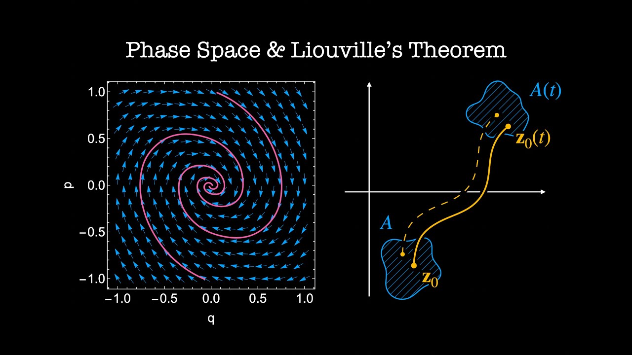
This image illustrates Liouville's theorem. On the right, a set of initial conditions occupying a region A evolves over time. The region deforms into a new shape A(t), but its volume (or area, in this 2D representation) remains constant: Volume(A) = Volume(A(t)). The vector field on the left depicts the phase space flow responsible for this evolution.

The shape of the region can, and often does, become fantastically distorted. A simple, compact shape like a sphere can be stretched into long, thin filaments that wind through phase space. However, the total volume occupied by these filaments will be exactly the same as the volume of the original sphere.

To see a concrete example of this stretching and squeezing, consider the simple (and non-physical, but illustrative) Hamiltonian $H = pq$ .

Classical Mechanics | Lecture 7

Professor Susskind analyzes the Hamiltonian H = pq, which causes exponential compression along the p-axis and exponential expansion along the q-axis, perfectly illustrating how the total phase space area is conserved while the shape changes dramatically.

Please watch this insightful example from the discussion.

This conservation of volume is a profound consequence of Hamiltonian dynamics. It implies that information is conserved. Since trajectories cannot merge (which would require a shrinking of volume), the system's evolution is reversible. If you know the state at time $t$ , you can uniquely determine the state at any past time.

This conservation law only holds for systems described by a Hamiltonian. Systems with dissipative forces, like friction, do not obey Liouville's theorem. In such systems, phase space volume shrinks, and trajectories can converge onto a single point (an attractor), losing information about their distinct origins.

Classical Mechanics | Lecture 7

To reinforce the conditions for the theorem, this final clip examines a system that violates it: the damped harmonic oscillator. The analysis shows that its phase space flow has a non-zero divergence, leading to a shrinking of phase space volume.

Watch the analysis of the damped harmonic oscillator. This will clarify why Hamiltonian structure is essential for Liouville's theorem to hold.

Conclusion

In this lesson, we have moved from a static to a dynamic picture of phase space and derived a fundamental law governing that motion.

Key Takeaways:

A statistical ensemble of systems can be pictured as an incompressible fluid flowing through phase space.
The velocity field of this fluid is determined by Hamilton's equations.
Liouville's theorem states that the divergence of this velocity field is zero ( $\nabla_{x} \cdot x ˙ = 0$ ). This is a direct consequence of the structure of Hamilton's equations.
The physical interpretation is that the volume of any region in phase space is conserved as it evolves in time. The shape of the region may change, but its volume does not.
This theorem is a statement about the conservation of information and reversibility inherent in Hamiltonian mechanics.

We now have a crucial piece of the puzzle: we know how a distribution of microstates evolves. But which distribution should we use? And how does this relate to the macroscopic properties we actually measure? To bridge this gap, our next lesson will introduce the ergodic hypothesis, a pivotal, though non-rigorous, assumption that connects time averages over a single system to ensemble averages over our phase space fluid. This will be the final step before we can formally construct the microcanonical ensemble.

Recommended resources

1. The Ensemble as a Fluid in Phase Space

2. The Divergence of the Phase Space Flow

3. Deriving Liouville's Theorem

4. Interpretation: Conservation of Phase Space Volume

Conclusion