Welcome to the third module of our course. Having explored kinetic theory and the approach to equilibrium, we now pivot to the central theme of our study: equilibrium statistical mechanics. Our goal in this and the coming modules is to build the entire structure of equilibrium thermodynamics from a few fundamental microscopic principles. This journey begins with establishing a precise language to connect the microscopic world of particles to the macroscopic world we observe.
In this lesson, we will define and relate three cornerstone concepts for a classical system of many particles: phase space, microstates, and macrostates. Understanding these ideas is the essential first step toward constructing statistical ensembles and deriving thermodynamic properties from first principles.
1. From Determinism to Statistics: Why We Need a New Approach
Your work with classical mechanics and simulations has shown you that, in principle, the evolution of a system of N particles is completely determined by Hamilton's equations, given a set of initial conditions. However, for a macroscopic system where , this deterministic approach becomes both practically impossible and conceptually unenlightening.
Professor Leonard Susskind opens his statistical mechanics course with a discussion of this very point.
Statistical Mechanics Lecture 1
This introductory clip from a Stanford lecture by Leonard Susskind explains why perfect predictability, while a feature of fundamental laws, is often useless for complex systems, motivating the turn to probability and statistics.
Please watch the segment from the introduction. He discusses the limitations of knowing initial conditions and the immense utility of statistical predictions for systems with a large number of components.
The issue is not just the sheer number of particles. Classical many-body systems are often chaotic. An infinitesimal uncertainty in the initial state can lead to exponentially divergent trajectories over time—the "butterfly effect." A deterministic prediction becomes meaningless after just a few collision times.
The following reading provides a striking quantitative illustration of this sensitivity.
These notes by D. Belitz offer a compelling argument for the necessity of a statistical description by analyzing the "spaghetti structure" of phase space.
Please read section 1.1.5, "Necessity of a Statistical Description of Many Particle Systems." Pay attention to the argument starting from the hard sphere collision, which calculates how quickly initial uncertainties are amplified. The discussion about the gravitational influence of a butterfly on a gas is particularly illuminating.
The conclusion is inescapable: for macroscopic systems, a deterministic, trajectory-by-trajectory description is a dead end. We must instead adopt a statistical approach, asking not "What is the precise state of the system?" but rather "What is the probability of finding the system in a certain state?" To formalize this, we first need to define the space of all possible states.
2. Phase Space: The Arena of Classical Dynamics
For a classical system, the complete instantaneous state is specified by the generalized coordinates and their conjugate momenta for all particles. Your study of advanced classical mechanics provides the necessary framework here.
For a system of particles moving in three dimensions, we have:
- position coordinates
- momentum coordinates
The phase space, often denoted by , is the -dimensional space spanned by these coordinates. A single point in this space, , represents the complete mechanical state of the entire system at a single instant in time. As the system evolves according to Hamilton's equations, this point traces a unique trajectory through phase space.
This section provides a formal definition of phase space within the Hamiltonian formulation of mechanics.
Please review section 1.1.1, "Hamilton’s Equations and Phase Space." Focus on the definition of phase space and the statement that an initial point uniquely determines the trajectory.
This -dimensional space is the stage upon which all of classical statistical mechanics unfolds. Every possible configuration and motion of the particles in the system is represented by a single point within it.
3. Microstates and Macrostates
With the concept of phase space established, we can now define the two most crucial terms in our statistical vocabulary.
-
A microstate is a single point in phase space. It is the most complete, detailed description possible for a classical system, specifying the position and momentum of every single particle.
-
A macrostate is a description of the system using a small number of macroscopic, measurable variables, such as total energy (E), volume (V), number of particles (N), pressure (P), and temperature (T).
The central idea of statistical mechanics is that a single macrostate corresponds to an immense number of different microstates. When we measure the pressure of a gas, we are not measuring the property of one specific microstate. Instead, we are observing a property that is an average over the countless microstates the system rapidly transitions through, all of which are consistent with the observed macrostate (e.g., all having the same total energy).
This brief section gives a clear and direct definition distinguishing microstates from macrostates.
Please read the introductory paragraphs of Section 1.3.1, "Statistical Description of Large Systems." The key distinction is made in the text starting from this sentence.
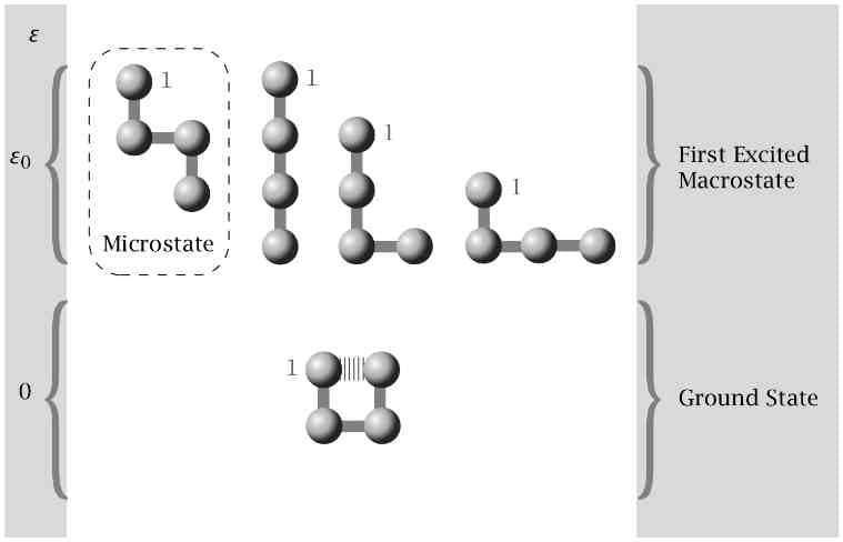
The relationship is illustrated below. Different microscopic configurations (microstates) of a polymer chain can have the same total energy, thereby belonging to the same macroscopic energy level (macrostate).
4. A Concrete Example: Counting States
To make these abstract definitions tangible, let's analyze a simple "toy model" where we can explicitly count the microstates for each macrostate. The following video provides an excellent, step-by-step walkthrough of this counting process.
Statistical Mechanics - Classical Statistics : Macrostates and Microstates
This video from the "Advanced Physics" channel uses the example of distributing four distinguishable particles into two compartments to clearly illustrate the difference between macrostates and microstates.
First, watch the introduction from the beginning, which sets up the problem for classical, distinguishable particles. Next, watch the segment defining and listing the macrostates, from the explanation. A macrostate here is defined by the number of particles in each of the two compartments (e.g., (4,0), (3,1), etc.). Finally, watch the detailed explanation of microstates from this point. This section shows how for a given macrostate, like (3,1), there are multiple distinct arrangements (microstates) of the labeled particles {A, B, C, D}.
Let's summarize the key results from the video for the system of 4 distinguishable particles (A,B,C,D) in 2 compartments:
| Macrostate (n₁, n₂) | Microstates (Specific arrangements) | Number of Microstates (Ω) |
|---|---|---|
| (4, 0) | {ABCD}, {} | 1 |
| (3, 1) | {ABC},{D}; {ABD},{C}; {ACD},{B}; {BCD},{A} | 4 |
| (2, 2) | {AB},{CD}; {AC},{BD}; {AD},{BC}; {BC},{AD}; {BD},{AC}; {CD},{AB} | 6 |
| (1, 3) | {A},{BCD}; {B},{ACD}; {C},{ABD}; {D},{ABC} | 4 |
| (4, 0) | {}, {ABCD} | 1 |
| Total | 16 = 2⁴ |
The number of microstates corresponding to a given macrostate, , is a fundamentally important quantity. It is often called the thermodynamic probability or statistical weight of that macrostate. As you saw in the video, this can be calculated using combinatorics. For a macrostate () where distinguishable particles are distributed among compartments, the number of microstates is given by the multinomial coefficient:
For our two-compartment example, this simplifies to the binomial coefficient . For the (2,2) macrostate, this gives , matching our explicit count.
Conclusion
In this lesson, we have laid the conceptual groundwork for equilibrium statistical mechanics. We have established that a deterministic approach is untenable for macroscopic systems and have defined the essential vocabulary to build a statistical framework.
Key Takeaways:
- Due to extreme sensitivity to initial conditions, a statistical description of many-particle systems is not just a convenience but a necessity.
- Phase space is the -dimensional space of positions and momenta that contains every possible mechanical state of a classical N-particle system.
- A microstate is a single point in phase space, representing a complete microscopic specification of the system.
- A macrostate is specified by a few macroscopic observables (like E, V, N).
- The core principle connecting these is that a single macrostate corresponds to a vast number of accessible microstates. The quantity , the number of microstates for a given macrostate, is called the thermodynamic probability.
We have so far treated microstates as static configurations. However, a real system is dynamic, constantly evolving from one microstate to another. In our next lesson, we will investigate how an entire collection of microstates, represented as a fluid-like distribution in phase space, evolves in time. This will lead us to Liouville's theorem, a crucial result that describes the conservation of phase-space volume and serves as the mechanical underpinning for the fundamental postulate of statistical mechanics.