Transport Coefficients from the Relaxation-Time Approximation

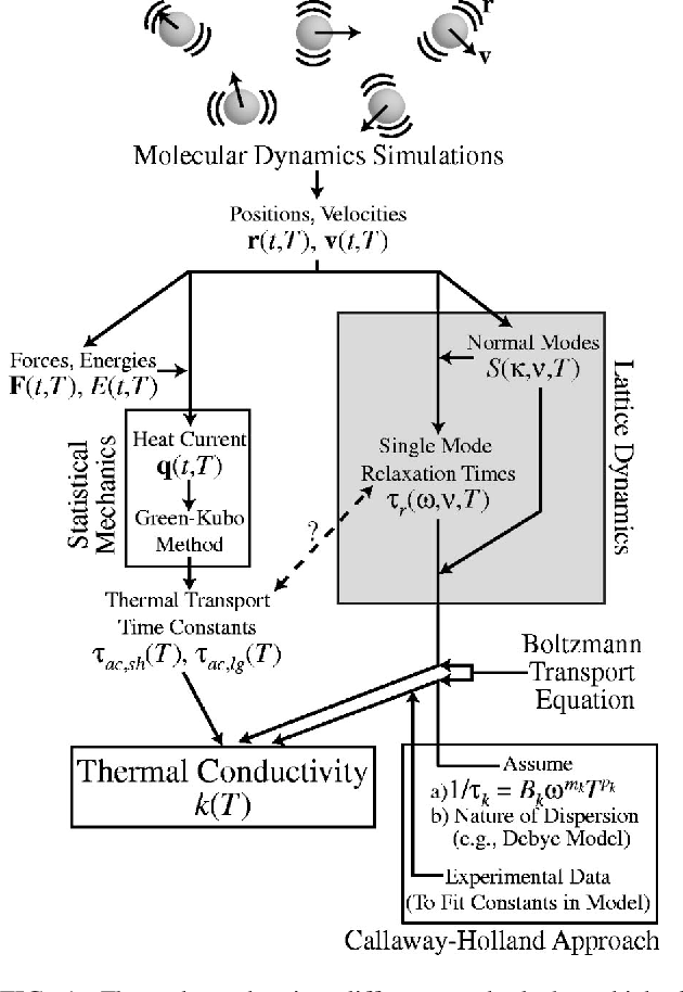
1. The General Principle of Flux Calculation

A transport process is fundamentally about the net flow, or flux, of a physical quantity like energy, momentum, or charge. For a quantity $A(\mathbf{p})$ carried by particles, the corresponding flux vector ${\mathbf{j}}_A$ is the average of $A(\mathbf{p})\mathbf{v}$ over the particle distribution:

A crucial simplification arises when we substitute $f=f_0+\delta f$. The local equilibrium distribution $f_0$ is isotropic in momentum (or velocity), meaning it's a function of energy $ϵ(p)=p^2/2m$ but not the direction of $\mathbf{p}$. Consequently, any integral of the form $\int (\dots )\mathbf{v}{f}_0{d}^{3}p$ must vanish, as for every particle with velocity $\mathbf{v}$, there is another with velocity $-\mathbf{v}$, leading to a perfect cancellation.

This means that a net flux can only arise from the anisotropic, non-equilibrium part of the distribution, $\delta f$.

This is the master formula for our lesson. By calculating this integral for energy and momentum, we will extract the thermal conductivity and viscosity, respectively.

2. Thermal Conductivity

Let's first derive Fourier's law of heat conduction. We consider a system in a steady state ($\partial /\partial t=0$) with a temperature gradient $\nabla T$ but no external forces ($\mathbf{F}=0$) and no bulk fluid motion ($\mathbf{u}=0$).

From our previous lesson, the steady-state BTE in the RTA gives:

Since temperature is the only spatially varying parameter affecting $f_0$, we use the chain rule:

This gives the specific form of the deviation for this problem:

The quantity being transported is thermal energy, $ϵ=\frac{1}{2}m{v}^2$. The heat current ${\mathbf{j}}_q$ is the flux of this energy. Its calculation involves a key integral over momentum space. The following video provides an exceptionally clear, step-by-step derivation, treating phonons as the energy carriers. The mathematical procedure is identical for gas molecules.

As demonstrated in the video, we calculate the component of the heat current along the gradient (let's say, in the z-direction, so $\nabla T=\frac{\partial T}{\partial z}\hat{\mathbf{z}}$):

This simplifies to:

Since the integral is over an isotropic equilibrium distribution, the average values of $v_x^2$, $v_y^2$, and $v_z^2$ are identical. Therefore, $⟨v_z^2⟩=\frac{1}{3}⟨v^2⟩$. We can replace $v_z^2$ with $\frac{1}{3}{v}^2$ inside the integral, which now becomes:

By comparing this to the phenomenological Fourier's law, $j_{q,z}=-\kappa \frac{\partial T}{\partial z}$, we can immediately identify the thermal conductivity, $\kappa$:

We can connect this rigorous result to the simpler formula from elementary kinetic theory. The heat capacity per unit volume is $C_V=\int ϵ(\partial f_0/\partial T)d^{3}p$. If we treat $\tau$ and $v^2$ as constants (a rough approximation), we can pull them out of the integral, yielding $\kappa \approx \frac{1}{3}{C}_V{v}^2\tau$. Recalling the mean free path $l=v\tau$, this becomes $\kappa \approx \frac{1}{3}{C}_{V}vl$, a familiar result. Our BTE derivation provides the proper way to average over the particle speeds and relaxation times.

To solidify this derivation, you can review it in a concise written format.

3. Shear Viscosity

Next, we derive Newton's law of viscosity. Here, the system is held at a constant temperature, but there is a gradient in the bulk fluid velocity. We consider a classic Couette flow where the fluid velocity is purely in the x-direction and varies only with the z-coordinate: $\mathbf{u}=u_x(z)\hat{\mathbf{x}}$.

In this scenario, the system is in local equilibrium, but the equilibrium distribution $f_0$ is centered on the non-zero local velocity $\mathbf{u}(\mathbf{r})$. For a classical gas, this is a displaced Maxwell-Boltzmann distribution:

The driving term for $\delta f$ is again $\mathbf{v}\cdot {\nabla }_{\mathbf{r}}{f}_0$. Applying the chain rule:

So, the deviation is:

Viscosity relates to the transport of momentum. The shear stress ${\Pi }_{zx}$ is defined as the flux of x-momentum ($p_x=m{v}_x$) in the z-direction.

The calculation proceeds very similarly to the one for thermal conductivity, involving an integral over the perturbed distribution. The MIT OCW video again provides an excellent guide through the mathematics.

Following the derivation, we substitute $\delta f$ into the integral for ${\Pi }_{zx}$:

By comparing with Newton's law of viscosity, ${\Pi }_{zx}=-\eta \frac{\partial u_x}{\partial z}$, we identify the shear viscosity, $\eta$. For an ideal gas, the integral evaluates to a remarkably simple expression:

where $n$ is the number density. This result is both elegant and powerful. For a concise written account of this derivation, refer to David Tong's notes.

4. A Note on Approximations

It is worth noting that the simple RTA we have used, where $\tau$ is a single constant, is a significant simplification. A more advanced treatment of the collision integral reveals that the relaxation process is more complex. For instance, the simple RTA predicts that the Prandtl number, a dimensionless ratio of momentum diffusivity (kinematic viscosity) to thermal diffusivity, Pr $=c_p\eta /\kappa$, is exactly 1 for a monatomic gas. Experimental values are closer to 2/3. This discrepancy is resolved by using more sophisticated models for the collision integral that go beyond the single relaxation time, but the RTA provides the correct qualitative dependencies and is an invaluable tool for physical insight.

Conclusion

In this lesson, we have bridged the gap between the microscopic and macroscopic worlds for transport phenomena. By combining the linearized Boltzmann equation with the relaxation-time approximation, we have moved beyond simple mean-free-path arguments to a systematic calculational framework.

Key Takeaways:

• Transport coefficients are proportionality constants that link a flux (of energy, momentum, etc.) to a thermodynamic driving force (a gradient in temperature, velocity, etc.).
• These coefficients can be derived by calculating the appropriate flux as a moment of the non-equilibrium part of the distribution function, $\delta f$.
• Thermal conductivity ($\kappa$) was found by calculating the energy flux driven by a temperature gradient, resulting in Fourier's Law.
• Shear viscosity ($\eta$) was found by calculating the momentum flux (stress tensor) driven by a velocity gradient, resulting in Newton's Law of Viscosity.
• The BTE-RTA method provides expressions for $\kappa$ and $\eta$ in terms of microscopic quantities like particle density, temperature, and, most importantly, the relaxation time $\tau$.

With this lesson, we conclude our module on kinetic theory. We have explored the microscopic origins of irreversibility and the approach to equilibrium, and we have developed a powerful tool to describe systems held in a steady, near-equilibrium state.

We will now shift our focus to the main subject of this course: equilibrium statistical mechanics. In the next lesson, we will lay the foundational postulates, starting with the concepts of phase space, microstates, and macrostates. We will introduce Liouville's theorem and the crucial, and subtle, ergodic hypothesis, which provides the ultimate justification for replacing impossibly complex time averages with much simpler ensemble averages. This will be our first step towards deriving all of equilibrium thermodynamics from a few fundamental principles.