DCF Model Components

The Big Picture: A Two-Stage Valuation Model

A DCF model seeks to determine a company's intrinsic value—its value based on its ability to generate cash. Since we assume a company will operate indefinitely (a "going concern"), we can't possibly forecast its cash flows forever.

To solve this, analysts use a two-stage model:

1. Stage 1: Explicit Forecast Period. This is a period, typically 5 to 10 years, for which we can create detailed, year-by-year financial forecasts.
2. Stage 2: Terminal Value. This is a lump-sum estimate of the company's value for all years beyond the explicit forecast period, based on an assumption of stable, long-term growth.

The company's total value is the sum of the present values of the cash flows from both stages.

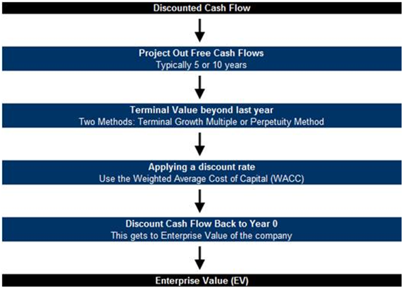
The flowchart below illustrates this entire process, from forecasting cash flows to arriving at the final value. We will now break down each of these steps.

Component 1: Forecasting Free Cash Flow to the Firm (FCFF)

The first and most critical component is the cash flow itself. In a DCF, we don't use net profit. Instead, we use Free Cash Flow (FCF), which represents the actual cash a company generates from its operations after paying for all operating expenses and investments.

Specifically, we use Unlevered Free Cash Flow, often called Free Cash Flow to the Firm (FCFF). This is the cash flow available to all of the company's capital providers—both debt holders (lenders) and equity holders (shareholders). By valuing this cash flow, we first arrive at the total value of the business operations, known as the Enterprise Value.

To understand what goes into calculating FCFF, please watch the following video segment.

As the video explained, the formula for FCFF is:

Let's break that down:

• EBIT(1 - Tax Rate): This is Earnings Before Interest and Taxes, adjusted for the cash taxes paid. It's a measure of operating profit.
• + D&A (Depreciation & Amortization): D&A is an accounting expense that reduces reported profit but doesn't actually use cash. We add it back to reverse this non-cash deduction.
• - Capital Expenditures (CapEx): This is the cash the company spends on long-term assets (like machinery or buildings) to maintain and grow its operations. This is a real cash outflow.
• - ΔNet Working Capital (Change in NWC): This represents the cash invested in the company's short-term operational needs, such as inventory and accounts receivable. An increase in NWC is a use of cash, so we subtract it.

Forecasting these components requires making detailed assumptions about the company's future, such as revenue growth and profit margins.

Component 2: The Discount Rate (WACC)

Once we have our forecasted FCFF for each year, we need a discount rate to bring them back to the present value. Since FCFF is the cash flow available to all capital providers, the discount rate must reflect the blended risk and required return of all of them.

This blended rate is the Weighted Average Cost of Capital (WACC).

Let's watch a short segment that introduces this concept.

The WACC formula looks like this:

Where:

• $E$ = Market Value of Equity
• $D$ = Market Value of Debt
• $K_e$ = Cost of Equity (the return shareholders require)
• $K_d$ = Cost of Debt (the interest rate the company pays on its debt)

Conceptually, the WACC is the average rate of return a company must pay to its investors (both shareholders and lenders) to finance its assets. We will explore exactly how to calculate this, particularly the Cost of Equity ($K_e$), in our next lesson.

Component 3: The Terminal Value (TV)

The Terminal Value (TV) is often the largest single component of a DCF valuation. It represents the value of the company for the entire period after our detailed 5-10 year forecast.

There are two primary methods to calculate it:

1. Perpetuity Growth Method: This assumes the company's cash flows will grow at a stable, constant rate ($g$) forever. The formula, also known as the Gordon Growth Model, is:

   $$\text{TV}=\frac{{\text{FCFF}}_{n+1}}{\text{WACC}-g}=\frac{{\text{FCFF}}_n\times (1+g)}{\text{WACC}-g}$$

   The growth rate ($g$) is typically a conservative estimate, often tied to the long-term GDP growth rate of the country.

2. Exit Multiple Method: This assumes the company is "sold" at the end of the forecast period (year n) for a multiple of a financial metric, like EBITDA.

   $$\text{TV}={\text{EBITDA}}_n\times \text{Exit Multiple}$$

   The multiple is usually based on what similar companies are trading at in the market.

To see these concepts explained in a real-world context for a Sri Lankan company, let's look at an introductory document for Alpha Fire Services Limited when it was listed on the CSE.

Putting It All Together: Enterprise Value to Equity Value

Now that we have all the components, we can assemble the valuation:

1. Calculate Present Value of Stage 1: Discount each of the explicit FCFFs from Stage 1 back to the present using the WACC.

   $$PV(\text{Stage 1})=\sum _{t=1}^n\frac{{\text{FCFF}}_t}{(1+\text{WACC}{)}^t}$$

2. Calculate Present Value of Stage 2: Calculate the Terminal Value (TV) at the end of the forecast period and discount that single lump-sum back to the present.

   $$PV(\text{Stage 2})=\frac{{\text{TV}}_n}{(1+\text{WACC}{)}^n}$$

3. Calculate Enterprise Value (EV): The sum of these two present values gives you the Enterprise Value.

   $$\text{Enterprise Value}=PV(\text{Stage 1})+PV(\text{Stage 2})$$

4. Bridge to Equity Value: The Enterprise Value is the value of the core business operations. To find the value that belongs just to shareholders (the Equity Value), we must adjust for non-operating assets and liabilities. The simplest way is:

   $$\text{Equity Value}=\text{Enterprise Value}-\text{Net Debt}$$

   Where Net Debt = Total Debt - Cash and Cash Equivalents.

5. Calculate Intrinsic Value per Share: Finally, to get the value per share, you divide the Equity Value by the number of diluted shares outstanding. You can then compare this intrinsic value to the current market price to decide if the stock is potentially undervalued or overvalued.

Conclusion

You have now seen the complete architecture of a Discounted Cash Flow model. It is a logical system built upon the time value of money, designed to convert a series of future cash flow expectations into a single present-day value.

Key Takeaways:

• A DCF model values a company based on the present value of its future cash flows.
• It uses a two-stage approach: an explicit forecast period and a Terminal Value.
• The three core components are:
  1. Free Cash Flow to the Firm (FCFF): The cash generated for all investors.
  2. Weighted Average Cost of Capital (WACC): The blended discount rate reflecting the risk to all investors.
  3. Terminal Value (TV): The estimated value of the company beyond the explicit forecast period.
• The DCF process calculates Enterprise Value first, which is then adjusted for net debt to arrive at Equity Value and a per-share intrinsic value.

Preview of the Next Lesson:

We've identified the WACC as the correct discount rate, but how do we calculate it? The WACC is highly sensitive to its inputs, especially the Cost of Equity ($K_e$). In our next lesson, we will focus on this critical component and learn how to estimate a company's required rate of return using the Capital Asset Pricing Model (CAPM) and beta.