Modeling and Forecasting Hotwife Intimacy Satisfaction with Brownian Motion

Welcome back. In our last lesson, we developed a robust statistical procedure for testing whether a sequence of discrete events, like 'peak photogenic moments', could be modeled by a Poisson process. We saw that when the model's assumptions don't hold, the nature of the failure itself provides valuable insight into the underlying dynamics.

Today, we transition from modeling discrete events in continuous time to modeling a variable that itself changes continuously and randomly. We will explore Brownian Motion, a cornerstone of stochastic processes. Your objective for this lesson is to calibrate a Brownian Motion model to represent the drift and volatility of the hotwife's intimacy satisfaction, and use it to forecast confidence intervals for future satisfaction levels.

This lesson will leverage your strong background in statistics, as we will frame the calibration problem as a parameter estimation task. We will translate the abstract concepts of drift and volatility into tangible metrics that describe the trajectory of relationship satisfaction, providing a powerful tool for both understanding and prediction.

1. Modeling Continuous Satisfaction with Brownian Motion

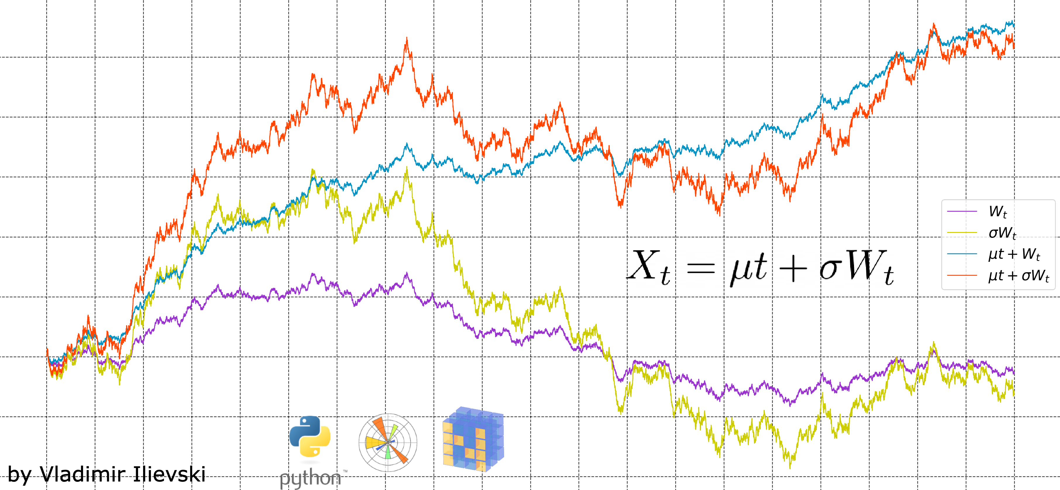
Imagine tracking the hotwife's overall satisfaction with her bull. Unlike discrete events (e.g., the number of encounters), satisfaction is a continuous quantity that fluctuates randomly from day to day, yet may also exhibit a general upward or downward trend over weeks or months. This is precisely the kind of phenomenon that Brownian Motion with drift is designed to model.

A standard Brownian Motion, often denoted $W_{t}$ , represents a pure, unbiased random walk. It has a mean of zero and a variance that grows linearly with time. However, to model real-world processes like satisfaction, we need to introduce two crucial parameters:

Drift ( $μ$ ): This parameter captures the deterministic, long-term trend. For intimacy satisfaction, a positive drift ( $μ > 0$ ) would signify a relationship that is, on average, growing stronger and more satisfying over time. A negative drift ( $μ < 0$ ) would suggest a gradual decline.
Volatility ( $σ$ ): This parameter captures the magnitude of the random, unpredictable fluctuations around the drift. High volatility means satisfaction levels can swing wildly from one day to the next, indicating an exciting but perhaps unstable dynamic. Low volatility implies a more predictable and stable level of satisfaction.

The combination of these elements gives us the model for Brownian Motion with drift, often expressed by the stochastic differential equation (SDE):

d X_{t} = μ d t + σ d W_{t}

Here, $d X_{t}$ represents the infinitesimal change in satisfaction $X$ over an infinitesimal time interval $d t$ . This change is composed of a deterministic part, $μ d t$ , and a random part, $σ d W_{t}$ . The integrated form of this equation shows how the satisfaction level $X_{t}$ at time $t$ evolves from an initial state $X_{0}$ :

X_{t} = X_{0} + μ t + σ W_{t}

This graph illustrates how the drift parameter ($\mu$) sets the overall direction of the process, while the volatility parameter ($\sigma$) determines the size of the random fluctuations around that trend.

To begin, let's formalize our understanding of these components.

Brownian Motion: A Study of Its Theory and Applications

This document provides a clear, non-technical introduction to the concepts of drift and volatility.

Please read the section titled "Subtlety Within Insanity." It introduces the equation for Brownian motion with these parameters, defining the process in terms of a standard Brownian Motion process X(t). Note that the author uses 'c' for volatility, which is equivalent to our \sigma. The key takeaway is how \mu governs the mean (the trend) and c (\sigma) governs the variance (the fluctuations).

2. Calibrating the Model from Data

To make this model useful, we must estimate $μ$ and $σ$ from real-world data. Let's assume the hotwife provides a daily satisfaction rating (e.g., on a scale of 0-100) for a period of $N$ days. This gives us a time series of observations: $X_{0}, X_{1}, X_{2}, \dots, X_{N}$ .

Our continuous model $d X_{t} = μ d t + σ d W_{t}$ can be approximated over discrete time steps. If our time step is $Δ t = 1$ day, the change in satisfaction from one day to the next, $Δ X_{i} = X_{i} - X_{i - 1}$ , can be modeled as:

Δ X_{i} \approx μ Δ t + σ Δ t Z_{i}

where $Z_{i}$ is a random variable drawn from a standard normal distribution, $Z_{i} \sim N (0, 1)$ .

This equation is fundamental. It tells us that the daily changes in satisfaction, $Δ X_{i}$ , should themselves be normally distributed with a mean of $μ Δ t$ and a variance of $σ^{2} Δ t$ .

Δ X_{i} \sim N (μ Δ t, σ^{2} Δ t)

With your background in statistics, you can see that this transforms our problem into a standard parameter estimation task. Given a sample of daily changes ${Δ X_{1}, \dots, Δ X_{N}}$ , we can estimate the mean and variance of the distribution they came from.

Estimate the Mean (Drift): The sample mean of the daily changes, $Δ X$ , is our best estimate for the theoretical mean, $μ Δ t$ . $μ^= \frac{Δ X}{Δ t}$
Estimate the Variance (Volatility): The sample variance of the daily changes, $s_{Δ X}^{2}$ , is our best estimate for the theoretical variance, $σ^{2} Δ t$ . $σ^^{2} = \frac{s _{Δ X}^{2}}{Δ t} ⟹ σ^= \frac{s _{Δ X}^{2}}{Δ t}$

This straightforward method is a form of Maximum Likelihood Estimation (MLE) for this discretized process. A more formal derivation involves constructing the joint probability density (the likelihood function) of the observed changes and finding the parameters $μ$ and $σ$ that maximize it.

[PDF] various parameter estimation techniques for stochastic differential ...

This thesis provides the mathematical foundation for this estimation procedure. It shows how the Euler-Maruyama discretization, which we've just used, allows us to construct an approximate likelihood function for the SDE.

Please read the section "Maximum Likelihood Estimation Technique" (4.1). Focus on the core idea, which starts by defining the likelihood function based on the transition PDF. The key insight is that this unknown PDF can be approximated by a normal distribution using the Euler-Maruyama approximation. The text then shows how this leads to explicit formulas for the estimators \hat{\alpha} (drift) and \hat{\beta} (squared diffusion) in equations (4.9) and (4.10), which are functionally identical to the method we just described.

As a crucial part of any statistical modeling, we should also verify the model's assumptions. In this case, we would need to test if the increments $Δ X_{i}$ are indeed independent and normally distributed. The same thesis outlines the relevant statistical tests (e.g., ADF test for stationarity, Shapiro-Wilk for normality, Box-Pierce for independence), which should be familiar territory for you.

3. Forecasting Future Satisfaction

Once we have our calibrated parameters, $μ^$ and $σ^$ , we can forecast future satisfaction levels.

Starting from the last observed satisfaction level, $X_{t}$ , the satisfaction at a future time $T$ is a random variable whose distribution is given by:

X_{T} ∣ X_{t} \sim N (X_{t} + μ^(T - t), σ^^{2} (T - t))

This powerful result gives us two things:

A Point Forecast: The expected value of future satisfaction is $E [X_{T}] = X_{t} + μ^(T - t)$ . This is simply the current satisfaction level projected forward along the estimated drift.
A Confidence Interval: Since we know the distribution is normal and we have its variance, we can construct a confidence interval. For example, a 95% confidence interval for $X_{T}$ is: $(X_{t} + μ^(T - t)) \pm 1.96 \cdot σ^T - t$

Notice how the width of the confidence interval grows with the square root of the forecast horizon ( $T - t$ ). This elegantly captures the fact that our uncertainty increases the further into the future we try to predict.

Let's apply this to the hotwife scenario:

Data: We have 91 daily satisfaction ratings, $X_{0}, \dots, X_{90}$ . The last rating is $X_{90} = 85$ .
Calibration: We compute the 90 daily changes $Δ X_{i}$ . We find their sample mean is $Δ X = + 0.2$ and their sample standard deviation is $s_{Δ X} = 3.0$ . With $Δ t = 1$ day, our parameters are:
- $μ^= 0.2$ (a small positive drift, indicating satisfaction is generally increasing by 0.2 points per day).
- $σ^= 3.0$ (a daily volatility of 3 points).
Forecasting: We want to forecast satisfaction 30 days from now (i.e., at $t = 120$ ).
- The forecast horizon is $T - t = 120 - 90 = 30$ days.
- Point Forecast: $E [X_{120}] = 85 + (0.2 \times 30) = 85 + 6 = 91$ .
- 95% Confidence Interval: $91 \pm 1.96 \times 3.0 \times 30 \approx 91 \pm 32.2$ . The interval is $[58.8, 123.2]$ . Since satisfaction is capped at 100, we would report the interval as $[58.8, 100]$ .

This forecast provides a tangible range of likely outcomes, quantifying both the expected growth and the inherent uncertainty in the relationship's trajectory.

To see this entire workflow applied in a published study, you can review the following example.

[PDF] various parameter estimation techniques for stochastic differential ...

This section of the thesis applies the exact methodology we've discussed to model the quantity of mandarin production over time.

Scan through the "Real Data example" (Section 5.2). Look at how the authors first check the assumptions (Tables 5.5, 5.6, 5.7), then present the estimated parameters in the final model (Equation 5.16), and finally, provide a forecast table (Table 5.9) and a corresponding graph (Figure 5.7) with confidence intervals. This is a perfect illustration of our learning outcome in practice.

4. Simulating Future Paths

Beyond generating a single forecast interval, our calibrated model allows us to simulate thousands of potential future paths for satisfaction. This can be extremely useful for understanding the range and nature of possible outcomes. The following video demonstrates how to implement a similar simulation in Excel for stock prices, which follow a closely related process called Geometric Brownian Motion.

Simulating Stock Price Paths with Random Walks in Excel / Analyzing stock returns / Episode 17

This tutorial from Initial Return provides a practical, step-by-step guide to simulating a stochastic process. While the specific formula is for Geometric BM (used for prices), the core steps of generating random shocks and iterating the process are identical.

Watch the following key segments: First, understand the inputs from the setup. This corresponds to our initial satisfaction level, \mu, and \sigma. Next, see how random shocks are generated using Excel functions from this section. This is the NORM.INV(RAND(), 0, 1) part, which creates our Z_i terms. Finally, observe how the iterative formula is built. The video uses S_{t+1} = S_t \times \exp(\dots) for Geometric BM. For our Arithmetic BM, the equivalent formula would be X_{t+1} = X_t + \hat{\mu}\Delta t + \hat{\sigma}\sqrt{\Delta t}Z_t. The principle is the same: each new value depends on the previous value plus a drift and a random shock.

Conclusion

In this lesson, we have seen how Brownian Motion with drift provides a quantitative framework for modeling and forecasting a continuous, randomly fluctuating variable like intimacy satisfaction.

Key Takeaways:

Brownian Motion with drift is characterized by two parameters: the drift $μ$ , which defines the long-term trend, and the volatility $σ$ , which defines the magnitude of random fluctuations.
These parameters can be estimated (calibrated) from a time series of historical data by calculating the mean and standard deviation of the observed increments.
Once calibrated, the model $X_{T} ∣ X_{t} \sim N (X_{t} + μ^(T - t), σ^^{2} (T - t))$ yields a full predictive distribution for future states.
This allows us to generate not only point forecasts but also statistically grounded confidence intervals, quantifying our uncertainty about the future.

In our next module, we will shift our focus from modeling the dynamics of satisfaction over time to identifying the drivers of a subjective outcome at a single point in time. Our first lesson will be to critique the Ordinary Least Squares (OLS) assumptions when modeling ordinal sexiness ratings and apply appropriate diagnostic tests. This will take us into the realm of regression, another powerful tool in your analytical arsenal.

Recommended resources

1. Modeling Continuous Satisfaction with Brownian Motion

2. Calibrating the Model from Data

3. Forecasting Future Satisfaction

4. Simulating Future Paths

Conclusion