Poisson Process for Peak Photogenic Moments

1. From Constant Rates to Time-Varying Intensity

Let's begin by quickly recapping the core relationship between the Exponential and Poisson distributions. A process of events is a (homogeneous) Poisson process if the waiting times between consecutive events are independent and exponentially distributed. This means the number of events occurring in any fixed time interval follows a Poisson distribution.

The core assumption of a homogeneous Poisson process is that the event rate, $\lambda$, is constant. For our boudoir photoshoot, this would mean "peak photogenic moments" are just as likely to occur at the beginning of the shoot as they are in the middle or at the end. This is a strong and often unrealistic assumption. A model's energy, creativity, and comfort with the photographer will naturally vary over time.

A more realistic model is the Nonhomogeneous Poisson Process (NHPP), or nonstationary Poisson process. Here, the constant rate $\lambda$ is replaced by a time-varying intensity function, $\lambda (t)$.

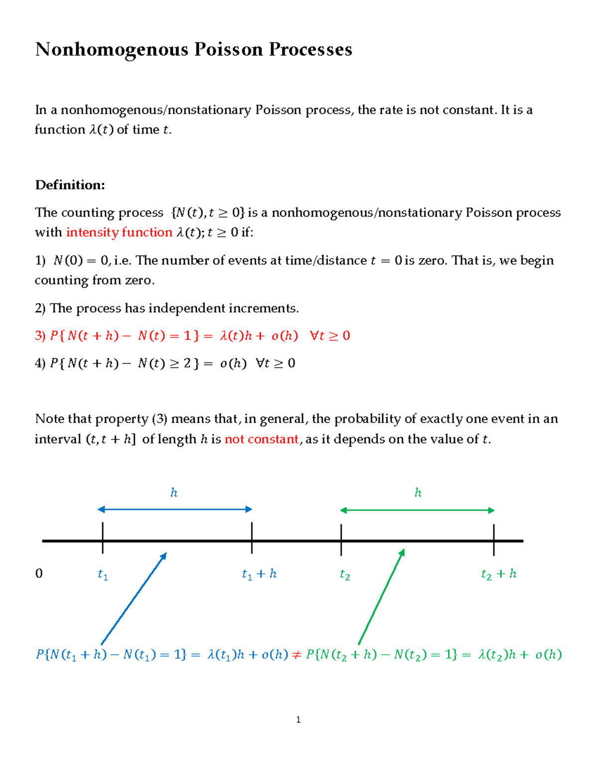
The NHPP elegantly captures the idea that the likelihood of a "peak moment" can rise as the model warms up, peak during a period of high energy, and then decline due to fatigue. Our central question is: given a set of timestamps for these peak moments, can we validate that they follow an NHPP?

2. A Strategy for Goodness-of-Fit Testing

To test if our data fits an NHPP, we need a method to handle the time-varying rate $\lambda (t)$. A powerful and practical approach is to approximate the continuous intensity function $\lambda (t)$ as being piecewise-constant (PC). We can break the total photoshoot duration (e.g., 2 hours) into smaller subintervals (e.g., 15-minute blocks) and assume the rate is constant within each block, though it can differ between blocks.

This simplifies the problem: instead of testing against a complex $\lambda (t)$, we test if the events within each subinterval follow a simple, homogeneous Poisson process. But how do we perform this test? This is where a clever transformation comes into play.

A foundational paper by Kim and Whitt, "Are Call Center and Hospital Arrivals Well Modeled by NHPPs?", outlines a robust methodology. While the paper is mathematically dense, its core ideas are highly practical.

The CU property is powerful, but a KS test applied directly to these transformed arrival times (the "CU KS test") has low power against one of the key alternative hypotheses: that the interarrival times are not exponentially distributed. To address this, we need a more targeted approach.

The assumption that arrivals in a subinterval follow a Poisson process has two distinct, testable components:

1. The interarrival times are exponentially distributed.
2. The interarrival times are independent and identically distributed (IID).

We therefore need to perform two separate statistical tests on the set of interarrival times within each subinterval.

3. Application: Diagnosing the Photoshoot Flow

Let's synthesize this into a concrete plan for our boudoir photoshoot scenario. Suppose we have the timestamps from a 90-minute shoot where the photographer marked every "peak photogenic moment."

Step 1: Partition the Data

First, we apply the piecewise-constant approximation. We divide the 90-minute session into six 15-minute subintervals. This choice involves a trade-off.

Step 2: Perform the Tests

For each of the six 15-minute intervals, we extract the list of interarrival times. Then, for each list, we perform our two hypothesis tests (e.g., at a 5% significance level):

• Test 1 (Exponentiality): The null hypothesis $H_0$ is that the interarrival times are exponentially distributed. We use a Lilliefors-corrected KS test. If the p-value is less than 0.05, we reject $H_0$.
• Test 2 (Independence): The null hypothesis $H_0$ is that the interarrival times are IID. We use a BDS test. If the p-value is less than 0.05, we reject $H_0$.

Step 3: Analyze the Implications

This is where the results become operationally meaningful. We can categorize each 15-minute subinterval based on the test outcomes.

• Case A: Both tests pass. The Poisson assumption holds for this interval. We can confidently estimate the rate ${\lambda }_i$ for this block. By comparing rates across blocks, we can identify the "golden hour" of the photoshoot—the period of highest creative output. Future shoots can be structured to place the most important outfits or poses within this high-$\lambda$ window.

• Case B: Exponentiality test fails, Independence test passes. This is a very common and insightful outcome. It means the process is not Poisson, but it is a more general renewal process. The waiting time for the next peak moment is not memoryless; it depends on the time elapsed since the last one.

  • Implication: This points to dynamics like a "warm-up" or "refractory" period after a successful shot. For example, the probability of the next peak moment might be low immediately after the last one, then increase over the next few minutes. This suggests modeling the interarrival times with a Weibull or Gamma distribution, as we alluded to in the last lesson. Operationally, it might mean the photographer should allow for short pauses after a flurry of great shots to let the creative energy "renew."

• Case C: Independence test fails. This implies that the length of one interarrival time predicts the length of the next. The process is not a renewal process.

  • Implication: This could signal momentum or fatigue. For example, a short interarrival time might be followed by another short one (positive autocorrelation), indicating the model is "in the zone." Conversely, a burst of activity (several short interarrival times) might lead to exhaustion, causing a subsequent long interarrival time (negative autocorrelation). This is a more complex process that cannot be modeled by simple renewal theory and may require time-series models that explicitly account for this dependence.

• Case D: Both tests fail. The process is neither Poisson nor a simple renewal process. The dynamics are complex, with both non-exponential waiting times and dependence between them.

The telemedicine thesis you read provides a perfect example of how these results are categorized.

Conclusion

In this lesson, we developed a practical, statistically robust procedure to test whether a sequence of events fits a Nonhomogeneous Poisson Process. By approximating the process as piecewise-constant and applying two targeted tests—the KS test for exponentiality and the BDS test for independence—we can not only validate the model but also gain deep insights from its failures.

Key Takeaways:

• To test if events follow an NHPP, we can partition the time into subintervals and test if each subinterval follows a homogeneous Poisson process.
• The Poisson assumption rests on two pillars: exponential interarrival times and independent interarrival times. These can be tested separately using the KS and BDS tests, respectively.
• If the exponentiality test fails, it suggests a more general renewal process where the hazard rate is not constant.
• If the independence test fails, it suggests a more complex process with memory between events, such as a time-series model.
• The outcome of these tests provides powerful diagnostic information to guide the selection of a more appropriate stochastic model for the process under study.

In our next lesson, we will shift gears from modeling discrete events to modeling continuous phenomena. We will learn how to calibrate a Brownian Motion model to represent the drift and volatility of the hotwife's intimacy satisfaction, and use it to forecast confidence intervals for future satisfaction levels. This will introduce a new set of tools for understanding systems that evolve continuously and randomly over time.