OLS Assumptions for Ordinal Data

1. The OLS Model and Its Foundational Assumptions

Ordinary Least Squares regression aims to find the best linear relationship between a set of independent variables (predictors) and a single dependent variable (outcome). In our photoshoot scenario, the goal would be to build a model like this:

Here, the coefficients ($\beta$) represent the estimated impact of each factor on the sexiness rating, and ${ϵ}_i$ is the error term, capturing all the unexplained variability. OLS works by finding the $\beta$ values that minimize the sum of the squared errors ($\sum {ϵ}_i^2$).

The reliability and validity of the OLS estimates depend on a set of critical assumptions about the data and the error term. For the OLS estimator to be the Best Linear Unbiased Estimator (BLUE), and for our statistical inferences (like p-values and confidence intervals) to be valid, these assumptions must hold.

2. The Critique: Modeling Ordinal Ratings with OLS

The central problem in applying OLS to our photoshoot scenario is the nature of the dependent variable: a "sexiness rating." This is an ordinal variable, not a continuous one. Let's say the ratings are on a scale of 1 (Not Sexy) to 5 (Very Sexy).

Applying OLS to such data is problematic for several reasons:

1. Arbitrary Distances: OLS assumes that the numerical distance between any two consecutive values is equal. It treats the difference between a rating of 1 and 2 as identical to the difference between 4 and 5. In reality, the perceived jump in "sexiness" might be very different across the scale.
2. Boundedness Violation: The outcome is bounded (1 to 5), but the linear model can predict values outside this range (e.g., a sexiness rating of 6.2 or -0.5), which is nonsensical.
3. Non-Normal Errors: The error term in a model with a discrete, bounded outcome is highly unlikely to follow a normal distribution, which invalidates standard hypothesis testing.

Using OLS in this context can lead to biased coefficient estimates and inaccurate conclusions about the significance of different outfits or poses.

3. Applying Diagnostic Tests to Reveal the Flaws

Even though we know OLS is theoretically inappropriate, let's proceed as if we were to use it anyway. The diagnostic tests, designed to check the OLS assumptions, will act as our "canary in the coal mine," revealing the problems created by the model-data mismatch.

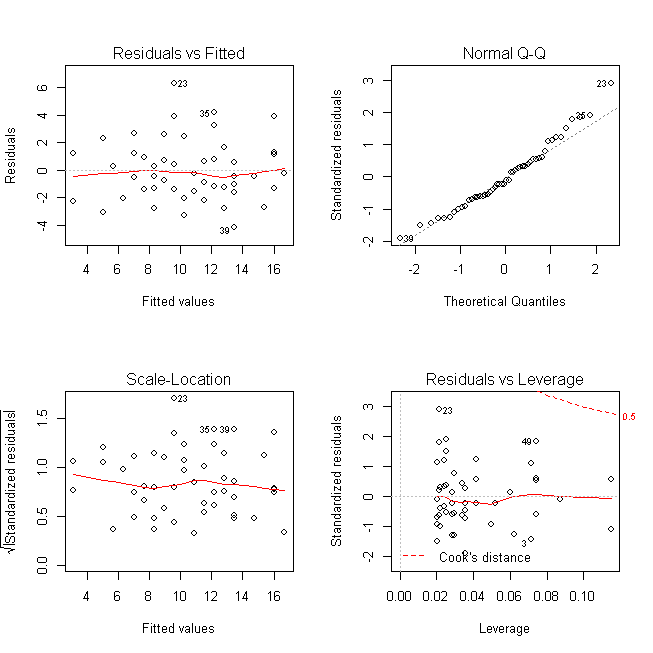
We'll examine the four key diagnostic plots, which are often generated automatically by statistical software.

A. Linearity and Independence

• Assumption: The relationship between predictors and the outcome is linear, and the errors are independent.
• Diagnostic: The Residuals vs. Fitted plot. For a good fit, we expect to see a random, formless cloud of points centered around zero.

In our scenario, because the SexinessRating can only take on a few integer values, the residuals ($e_i=y_i-{\hat{y}}_i$) will also be clustered into distinct horizontal bands. This is an immediate visual red flag that violates the "random cloud" expectation and hints at the non-continuous nature of our data.

The video below gives an excellent visual tour of how to interpret these plots.

B. Homoscedasticity (Constant Variance)

• Assumption: The variance of the errors is constant across all levels of the fitted values. This is known as homoscedasticity. The opposite, where the variance changes, is heteroscedasticity.
• Diagnostic: The Scale-Location plot (which plots $\sqrt{|\text{Standardized Residuals}|}$ vs. Fitted values) and formal statistical tests like the Breusch-Pagan test.

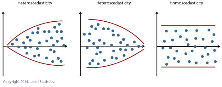
In our photoshoot model, it's plausible that there's more agreement (less variance) on what is not sexy (ratings near 1) and more disagreement (more variance) on what is very sexy (ratings near 5). This would create a funnel-shaped pattern in the residual plot, a classic sign of heteroscedasticity.

The Breusch-Pagan test formally checks for this by regressing the squared residuals on the independent variables. A significant p-value suggests heteroscedasticity.

For a more robust check, especially since you have a strong statistics background, the White test is superior to the Breusch-Pagan test. It checks for more general forms of heteroscedasticity by including not just the original predictors, but also their squares and cross-products in the auxiliary regression. This can detect non-linear relationships between the error variance and the predictors, which the Breusch-Pagan test might miss.

C. Normality of Residuals

• Assumption: The errors (${ϵ}_i$) are normally distributed. This is crucial for the validity of confidence intervals and hypothesis tests.
• Diagnostic: The Normal Q-Q (Quantile-Quantile) plot. If residuals are normal, the points should fall closely along the 45-degree reference line.

Given our ordinal outcome, the residuals will be discrete and bounded, not continuous and unbounded. Therefore, we should expect the Q-Q plot to show systematic deviations from the line, especially at the tails. This is another diagnostic that will fail precisely because of the nature of our dependent variable.

D. Outliers and Influential Points

• Concern: Some observations can have a disproportionate effect on the regression line.
• Diagnostic: The Residuals vs. Leverage plot and Cook's Distance. Leverage measures how unusual an observation's predictor values are, while Cook's Distance measures the overall influence of a single point on the model's coefficients.

In our photoshoot, a single, highly unusual outfit-pose combination that gets a very high or low rating could act as a high-leverage, high-influence point, warping the entire model. The diagnostics help us identify such cases.

Conclusion

In this lesson, we have critically examined the suitability of OLS regression for modeling ordinal outcomes like 'sexiness' ratings. We've seen that a theoretical mismatch exists and that this mismatch manifests as clear, detectable failures in standard OLS diagnostic tests.

Key Takeaways:

• OLS regression relies on several key assumptions, most fundamentally that the dependent variable is continuous.
• Applying OLS to an ordinal variable (like a 1-5 rating) is a methodological error that can lead to biased estimates and invalid statistical inference.
• The consequences of this error are not hidden; they are revealed by standard diagnostic tools. The Residuals vs. Fitted plot will show banding, the Scale-Location plot will likely show heteroscedasticity, and the Normal Q-Q plot will show non-normality.
• Formal statistical tests like the Breusch-Pagan or the more robust White test can confirm violations of the homoscedasticity assumption.

While we've demonstrated why OLS is the wrong tool for this job, you might wonder what the right tool is. The resource on "Ordinal Regression Models" introduces appropriate methods like the Ordered Logit model, which correctly handles the ordered, categorical nature of the data. While we won't delve into those models in this course, it is crucial to know they exist.

In our next lesson, we will pivot back to time-series analysis. You will apply Autoregressive Integrated Moving Average (ARIMA) to forecast cyclical patterns in the hotwife's desire and encounter frequency, and interpret the model's components. This will add another powerful forecasting method to your econometric toolkit, complementing the cross-sectional techniques we've discussed today.