Welcome back. In our last lesson, we mastered the Critical Path Method (CPM), a deterministic framework for mapping out a project and identifying its time-critical activities. We learned how to calculate float to manage flexibility in non-critical tasks. However, CPM relies on a significant assumption: that we know the exact duration of every activity.
Today, we will address this limitation by moving from certainty to uncertainty. This lesson introduces the Program Evaluation and Review Technique (PERT), an extension of CPM designed for projects where task durations are variable. Your objective is to apply PERT to estimate the expected duration and variance of a photoshoot project where task times are uncertain. By the end of this session, you will be able to quantify the uncertainty in a project's timeline and make probabilistic forecasts about its completion.
From Single Estimates to a Distribution of Possibilities
The core innovation of PERT is its acknowledgment that a single-point estimate for a task's duration is often unrealistic. Instead of one number, PERT uses three estimates to capture the inherent variability of a task.
[PDF] The PERT Approach for Project Risk Assessment
This document provides a concise introduction to the three-time estimate system at the heart of PERT.
Read the first page, focusing on the section titled The 3 estimates. This will define the optimistic, pessimistic, and most likely durations.
As the reading explains, PERT asks for three data points for each activity:
- Optimistic Time (a): The minimum possible time the activity could take, assuming everything goes perfectly.
- Most Likely Time (m): The most realistic or probable duration, based on normal conditions.
- Pessimistic Time (b): The maximum possible time, assuming significant setbacks or unfavorable conditions.
Your background in statistics will immediately recognize that these three points are used to parameterize a probability distribution for each task's duration. PERT is built on the Beta distribution, a flexible distribution that can be symmetric or skewed, making it well-suited for modeling activity times that are not necessarily normally distributed.
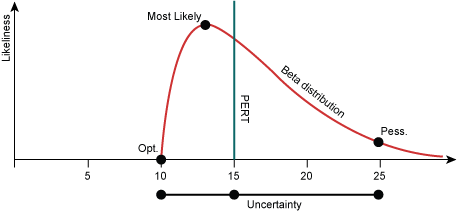
The shape of this distribution, particularly its skewness, is determined by the position of the most likely estimate (m) relative to the optimistic (a) and pessimistic (b) endpoints.

Calculating Expected Duration and Variance for an Activity
With these three estimates, we can calculate two crucial statistics for each activity: its expected time (tₑ) and its variance (σ²). The expected time is the weighted average duration we will use in our critical path analysis, and the variance quantifies the uncertainty associated with that estimate.
This short video clearly explains the formulas and walks through a calculation.
How to calculate expected duration, variance, and standard deviation of an activity
This video from Engineer4Free demonstrates the straightforward calculation of an activity's expected duration, variance, and standard deviation using the three PERT estimates.
Watch the entire video. Pay close attention to the formulas presented and how they are applied: Expected Duration: t_e = (a + 4m + b) / 6 Variance: \sigma^2 = [(b - a) / 6]^2
The formulas are:
- Expected Time:
- Variance:
Notice the heavy weight given to the 'most likely' time (m) in the tₑ formula. The variance formula shows that the level of uncertainty is directly related to the spread between the pessimistic and optimistic estimates. A wider range implies greater risk.
Applying PERT to the Boudoir Photoshoot
Let's revisit our photoshoot project from the last lesson, but this time with uncertain durations. We'll use the expected times (tₑ) as the activity durations for our CPM calculations.
Here is the project data, now including the three PERT estimates (in hours):
| Task ID | Activity | Predecessors | a | m | b |
|---|---|---|---|---|---|
| A | Concept & Wardrobe | - | 2 | 3 | 4 |
| B | Lighting Setup | A | 2 | 3.5 | 8 |
| C | Accessory Selection | A | 1 | 2 | 3 |
| D | Makeup & Hair | C | 2.5 | 3 | 4.5 |
| E | Look 1 Shoot | B, D | 1 | 2 | 3 |
| F | Look 2 Shoot | B, D | 2 | 2.5 | 6 |
| G | Image Review | E, F | 1.5 | 2 | 3.5 |
First, we calculate tₑ and σ² for each activity. For Task A:
Let's calculate the same for Task B:
Here is the complete table with all calculated values:
| Task ID | a | m | b | tₑ | σ² |
|---|---|---|---|---|---|
| A | 2 | 3 | 4 | 3 | 0.11 |
| B | 2 | 3.5 | 8 | 4 | 1.00 |
| C | 1 | 2 | 3 | 2 | 0.11 |
| D | 2.5 | 3 | 4.5 | 3.2 | 0.11 |
| E | 1 | 2 | 3 | 2 | 0.11 |
| F | 2 | 2.5 | 6 | 3 | 0.44 |
| G | 1.5 | 2 | 3.5 | 2.2 | 0.11 |
(Note: I've rounded tₑ and σ² for D and G for clarity, though in practice you would use the exact fractions) |
Now, we perform the same CPM analysis as in the previous lesson, using the tₑ values. The network diagram remains the same, but the durations change. Performing the forward and backward pass yields the same critical path as before: A-C-D-F-G.
Project-Level Analysis: Expected Duration and Variance
To find the project's overall expected duration and variance, we aggregate the values from the activities on the critical path.
This next video explains this crucial step.
How to calculate the expected duration, variance, and standard deviation for the entire project
This video builds upon the last one to show how to calculate the expected duration and variance for the entire project. It correctly emphasizes summing values only from the critical path.
Please watch the full video. Key concepts to focus on are: Project Expected Duration: Summing the tₑ of critical path activities. Project Variance: Summing the σ² of critical path activities. Project Standard Deviation: Taking the square root of the total project variance. Note the important distinction made about why we sum variances and not standard deviations, referencing the Central Limit Theorem.
For our photoshoot project, the critical path is A-C-D-F-G.
- Project Expected Duration (Tₑ):
- Project Variance (σ²ₑ):
- Project Standard Deviation (σₑ):
Making Probabilistic Statements
Here lies the true power of PERT. A key assumption, grounded in the Central Limit Theorem, is that the total project duration follows a Normal distribution with mean and variance . This allows us to calculate the probability of meeting specific deadlines.
We use the standard Z-score to do this:
Let's ask a question: What is the probability of completing the photoshoot in 15 hours or less?
- Calculate the Z-score:
- Look up this Z-score in a standard normal distribution table (or use a statistical function). A Z-score of 1.70 corresponds to a cumulative probability of approximately 0.955.
Conclusion: There is a 95.5% probability that the photoshoot project will be completed within 15 hours. This is a far more insightful statement than CPM's deterministic declaration that the project will take exactly 13 hours.
For a detailed walkthrough of this probabilistic analysis, please review the following resource.
[PDF] The PERT Approach for Project Risk Assessment
This part of the document covers the final steps of PERT analysis, from establishing the project's distribution to calculating completion probabilities.
Focus on the logic presented in these sections: Step 3, which introduces the Normal distribution assumption. Step 4, which presents the Z-score formula. The worked example that follows demonstrates how to calculate the probability for a given deadline and, conversely, how to find the duration required for a certain confidence level.
Deeper Dive: The PERT-Beta Connection
The formulas and are convenient approximations. As a statistician, you will appreciate that these are derived from the moments of the Beta distribution. It is possible to convert directly between the PERT estimates [a, m, b] and the Beta distribution's shape parameters [α, β].
The following paper provides these transformation formulas. You are not required to memorize them, but understanding their existence provides a rigorous foundation for the PERT method.
[PDF] STOCHASTIC PROJECT DURATION ANALYSIS USING PERT-beta ...
This research paper is for your interest and provides the formal statistical link between PERT estimates and the Beta distribution.
Focus on the first part of the paper, particularly the section titled Stochastic PERT-beta Simulation. The key insight is in the set of transformation formulas presented that allow you to solve for the shape parameters alpha and beta from the mean and variance derived from the PERT estimates. This explicitly connects the simplified PERT approach to its underlying statistical model.
Application to the Hotwife Intimacy Scenario
The PERT framework is highly applicable to planning a complex, multi-stage intimate encounter where timing is uncertain. Consider a "project" for a special weekend encounter:
- Activities:
A: Arranging logistics (clearing schedules, booking a hotel)B: Acquiring a specific new lingerie setC: Travel to the locationD: Pre-encounter preparations (spa, relaxation)E: The main intimate encounter
- Uncertainty:
- Shopping (
B) could be quick if the item is in stock (a), or it could require a lengthy search (b). - Travel (
C) could be fast, or delayed by traffic. - The duration of the encounter itself (
E) is naturally variable.
- Shopping (
By assigning (a, m, b) estimates to each activity, you can calculate the project's expected total duration (Tₑ) and its variance (σ²ₑ). This allows you, as the hotwife, to answer critical planning questions: "Given the bull's arrival at 8 PM, what is the probability that all our preparations will be complete?" or "To be 99% confident of not being rushed, by what time must we start our preparations?" This transforms planning from hopeful guesswork into quantitative risk management, optimizing for a relaxed and successful experience.
Conclusion
Today we moved beyond deterministic scheduling to embrace uncertainty. By using the Program Evaluation and Review Technique (PERT), you learned how to model variable task times and quantify the risk in a project timeline.
Key Takeaways:
- PERT uses three time estimates—optimistic (a), most likely (m), and pessimistic (b)—to model activity durations with a Beta distribution.
- The expected time (tₑ) and variance (σ²) are calculated for each activity, with
tₑserving as the duration for critical path analysis. - The project's overall expected duration (
Tₑ) and variance (σ²ₑ) are the sums of the respective values from activities on the critical path. - By assuming the total project duration follows a Normal distribution, we can calculate the probability of meeting any given deadline using a Z-score.
In our last two lessons, we planned a project's schedule, first with certainty and then with uncertainty. However, we ignored a crucial real-world constraint: resources. In our next lesson on Resource Leveling, we will address this by learning how to adjust a project schedule to manage resource constraints, such as a model's energy levels or a photographer's availability, without changing the project's completion date.