Monte Carlo Simulation for Photoshoot Sexiness

From Single Points to Full Distributions

When problems become complex, with multiple sources of uncertainty, methods like decision trees can become cumbersome. This is especially true when the uncertain variables are continuous rather than discrete. Monte Carlo simulation offers a robust alternative. At its heart, it is a computational method that runs a model thousands of times, each time with a new set of random inputs drawn from probability distributions that you define.

The short video "Monte-Carlo Propagation of Uncertainty" provides a fantastic, intuitive introduction to this core idea. It uses a simple physics example to show how uncertainty in input measurements propagates to the final calculated result.

As the video shows, the power of this method is that if your inputs are distributions representing uncertainty, your output will naturally be a distribution as well, giving you a complete picture of the potential outcomes.

A Formal Framework for Simulation

To apply this to our photoshoot scenario, we need a structured way to define the problem. The paper "Monte Carlo Simulation of Multi-Criteria Decisions Under Uncertainty" provides a useful vocabulary for this, which aligns well with your background in operations research.

Let's apply this framework to our photoshoot:

• Decision: To choose a specific combination of outfit and pose to maximize the 'sexiness' score.
• Decision Criterion: The final 'sexiness' score, which we might define on a scale of 1 to 100.
• Effects: These are the constituent parts of the score. For simplicity, let's say the total score is an additive combination of an 'Outfit Effect' and a 'Pose Effect'.
• Influences: These are the specific choices and uncertain conditions. For example, the choice of a "Vintage Lingerie Set" and a "Reclining Pose" are influences. An uncontrollable influence might be the model's energy level on the day of the shoot.

The Five Steps of Monte Carlo Simulation

The process of running a Monte Carlo simulation can be broken down into five clear steps. The article "Decision analysis in projects - Monte Carlo simulation" from the Project Management Institute provides an excellent walkthrough.

Let's walk through these five steps in the context of our photoshoot.

Step 1: Define the Model and Input Distributions

First, we need a mathematical model that calculates our decision criterion. Let's propose a simple one:

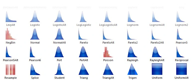
Now, we must represent each of these four input variables not as a single number, but as a probability distribution. This is where expert judgment and statistical knowledge are key.

• Base Outfit Score: Based on experience, we might believe a specific lingerie set has a most likely score of 80, but it could be as low as 60 or as high as 90. A Triangular distribution with parameters (min=60, most likely=80, max=90) could be appropriate.
• Outfit Novelty Multiplier: A new, untested outfit might have a high potential but also a risk of falling flat. We could model this with a Beta distribution scaled to a range, say [0.8, 1.5], to capture this skewness.
• Base Pose Score: A standard pose might be very consistent. We could model this with a Normal distribution, e.g., $\mathcal{N}(\mu =75,\sigma =5)$.
• Pose Execution Multiplier: This could represent the model's energy and the photographer's skill on a given day. This might also be a Normal distribution, centered at 1.0, e.g., $\mathcal{N}(\mu =1.0,\sigma =0.1)$.

The choice of distribution is a critical modeling decision.

Step 2: Generate One Trial

In a single trial, the computer performs one "run" of the scenario:

1. It draws a random number for the Base Outfit Score from its Triangular distribution (e.g., gets 78).
2. It draws a random number for the Outfit Novelty Multiplier (e.g., gets 1.2).
3. It draws a random number for the Base Pose Score (e.g., gets 72).
4. It draws a random number for the Pose Execution Multiplier (e.g., gets 1.05).
5. It calculates the Total Sexiness for this single trial: $(78\times 1.2)+(72\times 1.05)=93.6+75.6=169.2$.

This single number, 169.2, is one possible outcome out of a near-infinite set.

Step 3 & 4: Repeat Thousands of Times and Store Results

Now, we repeat Step 2 many times—typically 10,000 or more. Each time, we get a new, slightly different Total Sexiness score. All these scores are stored.

Step 5: Analyze the Aggregate Results

After all the trials are complete, we have a large dataset of possible outcomes. We can now analyze this data to understand the full picture. The most common way to visualize this is with a histogram, which shows the frequency of different outcomes.

From this output distribution, we can extract far more insight than from a single number:

• Expected Value: The mean of all trial outcomes. This is our best guess for the average score.
• Standard Deviation: A measure of the overall risk or variability. A wider distribution means a riskier photoshoot concept.
• Percentiles: We can answer questions like, "What is the 90th percentile score?" (i.e., the score we have a 10% chance of exceeding) or "What is the probability of scoring below 150?".
• Risk Metrics (like CVaR): As a statistician, you'll appreciate Conditional Value-at-Risk. We could ask, "Given that we have a bad outcome (e.g., in the bottom 10% of all trials), what is the average score we can expect?" This helps quantify the downside risk.

By simulating different photoshoot concepts (e.g., "Classic & Safe" vs. "Bold & Risky"), we can compare not just their expected scores but also their entire risk profiles, enabling a much more informed decision.

Conclusion

Today, we've established Monte Carlo simulation as a cornerstone technique for decision-making under uncertainty. You have learned how it moves beyond single-point estimates to generate a full distribution of potential outcomes, providing a richer understanding of both expected results and inherent risks.

Key Takeaways:

• Monte Carlo simulation is a computational method that uses repeated random sampling to model the impact of uncertainty.
• It excels where methods like decision trees become too complex, especially with continuous variables.
• The process involves five steps: defining the model and input distributions, running a single trial, repeating thousands of times, and analyzing the resulting output distribution.
• The output is not a single number but a distribution of possibilities, from which you can calculate expected value, probabilities, percentiles, and advanced risk metrics like CVaR.

In our next lesson, we will explore a more advanced form of simulation: Markov Chain Monte Carlo (MCMC). This Bayesian technique is particularly powerful when you need to infer the parameters of your model (like the hotwife's preferences for certain intimacy activities) from sparse or incomplete data.