MCMC for Hotwife Preference Estimation

The Bayesian Inference Problem: From Prior Beliefs to Posterior Knowledge

At its core, your task is to learn about a set of unknown parameters—in this case, the hotwife's "true" preference scores for various intimacy activities—using limited data. As a statistician, you are familiar with the Bayesian framework:

1. Prior Distribution: We start with initial beliefs about the parameters. For instance, we might assume her preference for any new activity is, on average, a 7 out of 10, with some uncertainty. This is our prior, $P(\theta )$.
2. Likelihood: We define a model for how the observed data (e.g., her satisfaction ratings after an encounter) depends on the unknown preference scores. This is the likelihood, $P(\text{data}|\theta )$.
3. Posterior Distribution: We use Bayes' theorem to combine our prior beliefs with the evidence from the data to get an updated understanding of the parameters. This is the posterior, $P(\theta |\text{data})$.

The challenge lies in computing the posterior. The denominator, $P(\text{data})$, known as the marginal likelihood or evidence, involves integrating over all possible parameter values. For any non-trivial model, this integral is computationally intractable. This is where MCMC comes in.

The following video provides an excellent high-level introduction to Bayesian inference and motivates the need for MCMC.

The key takeaway is that MCMC methods don't solve the integral analytically. Instead, they provide a clever way to generate a large number of samples that are, in effect, drawn directly from the posterior distribution. By analyzing these samples, we can approximate any property of the posterior we care about (mean, variance, credible intervals, etc.).

How MCMC Works: The Metropolis-Hastings Algorithm

So, how do we generate samples from a distribution we can't even write down in a closed form? The most famous MCMC algorithm is Metropolis-Hastings. It constructs a Markov chain—a sequence of random variables where the next state depends only on the current state—whose "stationary distribution" is precisely the posterior distribution we want to sample from.

The process is remarkably elegant and can be broken down into a simple loop:

1. Start at some initial parameter value, ${\theta }_t$.
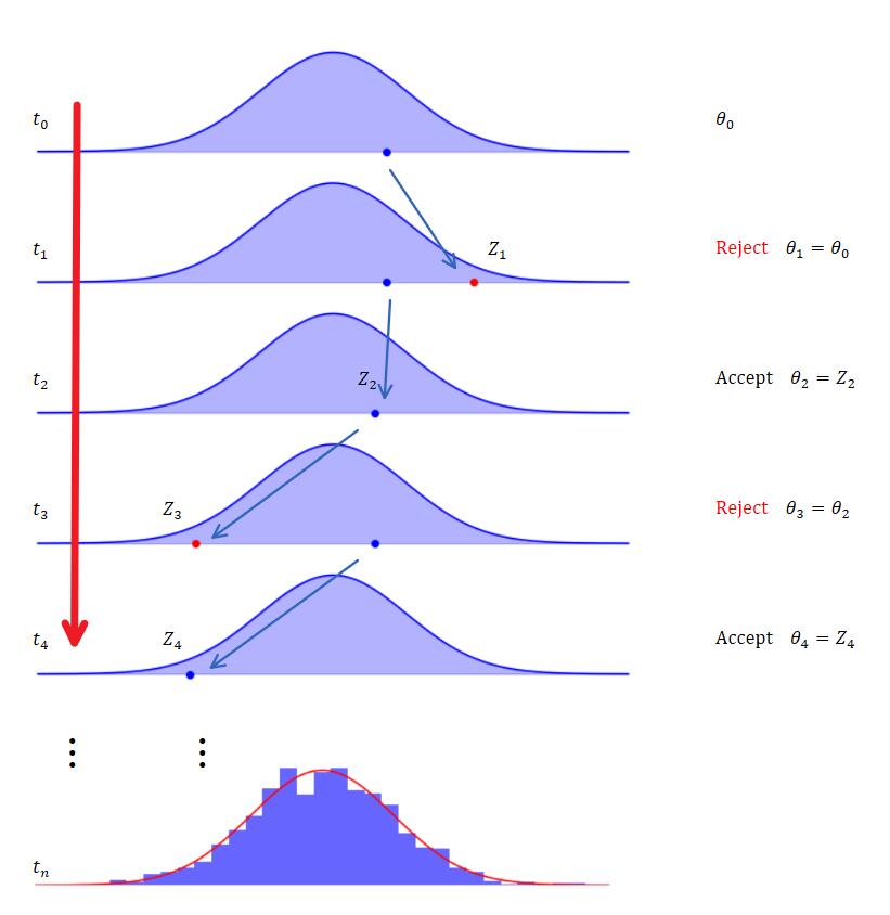
2. Propose a new value, ${\theta }^{\prime }$, from a proposal distribution centered on the current value (e.g., a normal distribution, $\mathcal{N}({\theta }_t,{\sigma }^2)$).
3. Calculate an acceptance probability, which compares how plausible the new state ${\theta }^{\prime }$ is compared to the current state ${\theta }_t$, according to the posterior distribution.
4. Accept or Reject: Draw a random number. If it's below the acceptance probability, move to the new state (${\theta }_{t+1}={\theta }^{\prime }$). Otherwise, stay put (${\theta }_{t+1}={\theta }_t$).
5. Repeat.

This simple "propose-and-decide" process, when repeated thousands of times, generates a "chain" of parameter values. After an initial "burn-in" period, the samples in this chain are valid draws from the posterior distribution.

The video below gives a fantastic and intuitive walkthrough of the mechanics and logic of the Metropolis-Hastings algorithm.

The image below illustrates this iterative process. At each step, a new candidate value $Z_i$ is proposed. The algorithm decides whether to accept this new value as the next state in the chain or to reject it and stay at the current state. Over many iterations, the collection of accepted states (the histogram at the bottom) builds up to approximate the target posterior distribution.

Application: Inferring Intimacy Preferences from Sparse Data

Now, let's apply this to the hotwife scenario. Imagine she wants to understand her preferences for a set of different intimacy activities, say:

• A: Quick, spontaneous encounter
• B: Planned, romantic date night
• C: Experimental roleplay session
• D: Long, sensual massage

The "parameters" we want to infer are her latent preference scores for each, ${\theta }_A,{\theta }_B,{\theta }_C,{\theta }_D$. The "data" is sparse feedback—perhaps a few satisfaction ratings (e.g., "Encounter type B was an 8/10") and some pairwise comparisons ("The last A was more satisfying than the C before it").

If we treat each ${\theta }_i$ as independent (a "no pooling" model), we have a problem. If she's only tried roleplay (C) once, our estimate for ${\theta }_C$ will have huge uncertainty. This is where hierarchical models, a natural partner to MCMC, become incredibly powerful.

Instead of assuming each ${\theta }_i$ is completely independent, we can model them as being drawn from a common parent distribution:

Here, $\mu$ represents her overall "average preference for intimacy," and ${\sigma }^2$ represents how much her preferences vary across different activities. In this setup, an activity with sparse data can "borrow strength" from the others. The model uses information from activities B and D to inform its estimate for C.

MCMC is the engine that makes this work. We don't just estimate the ${\theta }_i$s; we also estimate the hierarchical parameters $\mu$ and ${\sigma }^2$ at the same time. The model learns the appropriate amount of "pooling" or information sharing directly from the data.

The Faculty video you watched earlier explains this concept of partial pooling brilliantly. Let's revisit a key segment.

A Practical Implementation: The Bayesian Mallows Model

To make this even more concrete, let's look at a specific model designed for preference and ranking data: the Mallows rank model. It defines a probability distribution over the space of all possible rankings of a set of items. The distribution has two main parameters:

• $\rho$: The latent consensus ranking, which represents the single ranking that is most likely to be the "true" preference order. In our case, this would be the hotwife's ideal ranking of activities A, B, C, and D.
• $\alpha$: A scale parameter that controls the concentration. A high $\alpha$ means most observed rankings are very close to the consensus $\rho$. A low $\alpha$ means there's a lot of variation or uncertainty in the rankings.

The following presentation provides a brief but excellent overview of using a Bayesian MCMC approach to fit a Mallows model, which is perfectly suited to our problem of inferring preferences from sparse data.

This framework, as detailed in the underlying research paper "Probabilistic Preference Learning with the Mallows Rank Model" (ID: LINK), uses data augmentation within the MCMC algorithm. It treats the missing parts of the rankings as parameters to be estimated, allowing it to elegantly handle the sparse feedback that characterizes our problem.

Interpreting the MCMC Output

After running the MCMC algorithm for, say, 20,000 iterations, we get a chain of samples for each parameter. Before analysis, we must:

1. Discard the burn-in: The initial samples are discarded because the chain has not yet converged to the stationary distribution.
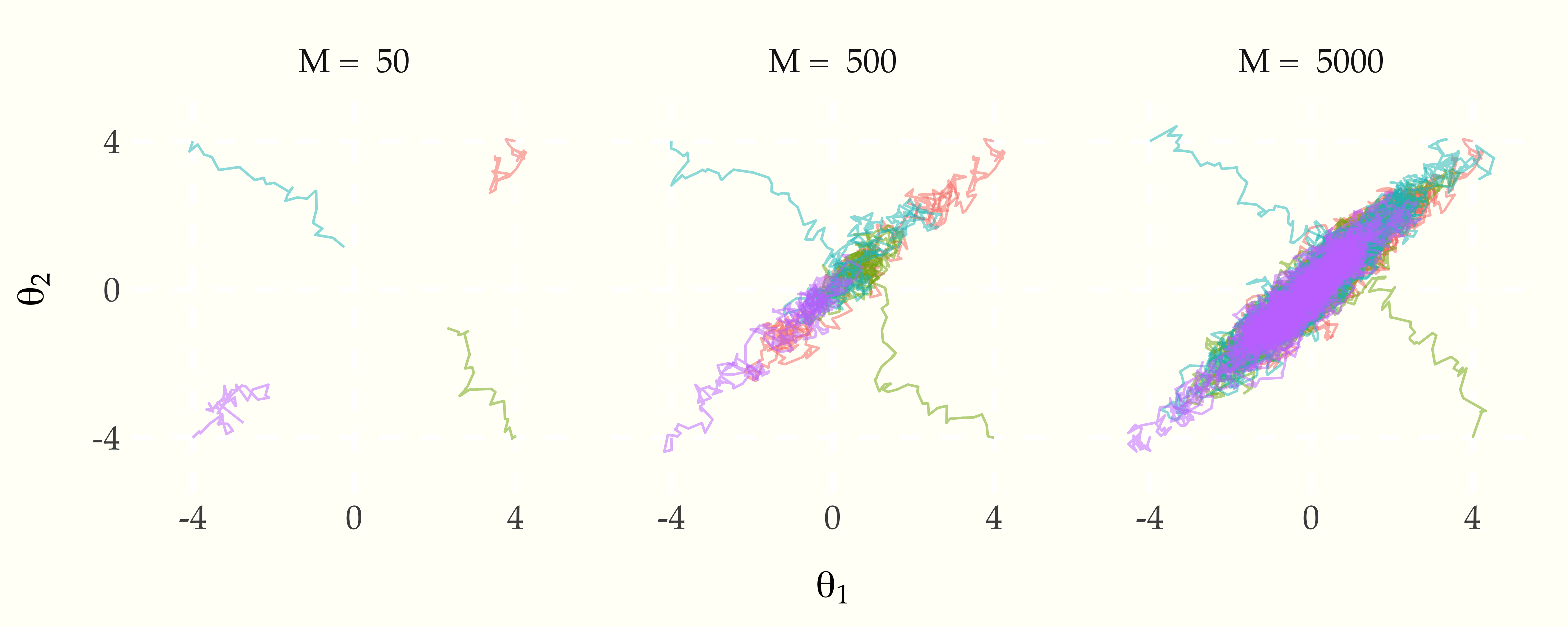
2. Check for convergence: We typically run multiple chains from different starting points. If the algorithm is working correctly, all chains should forget their starting points and converge to sample from the same posterior distribution. This is called "mixing."

The image below shows several MCMC chains exploring a two-dimensional parameter space. Initially, the chains explore different regions, but as the number of iterations (M) increases, they all converge and sample from the same high-probability area, which represents the posterior distribution.

Once we have our converged samples, we can analyze them to answer our questions. For each intimacy activity, we don't get a single preference score; we get a full posterior distribution. We can then calculate the mean preference, a 95% credible interval, or answer probabilistic questions like: "What is the probability that 'Experimental Roleplay' (${\theta }_C$) is more preferred than 'Planned Date Night' (${\theta }_B$)?" We would answer this by simply counting the proportion of samples in our MCMC output where the sampled value for ${\theta }_C$ was greater than the sampled value for ${\theta }_B$.

Conclusion

In this lesson, we've journeyed from the "what-if" analysis of Monte Carlo simulation to the inferential powerhouse of Markov Chain Monte Carlo. You have seen how MCMC provides a computational solution to the often intractable problem of Bayesian inference, allowing us to learn about unknown parameters from limited and noisy data.

Key Takeaways:

• MCMC is a class of algorithms used to sample from a probability distribution, particularly the posterior distribution in Bayesian analysis, when it cannot be computed directly.
• The Metropolis-Hastings algorithm provides a simple but powerful mechanism to construct a Markov chain that converges to the desired posterior distribution by iteratively proposing and accepting/rejecting new states.
• For problems with sparse data across multiple groups (like estimating preferences for different intimacy activities), combining MCMC with hierarchical models allows for "partial pooling," where groups with little data can borrow statistical strength from those with more data.
• The output of an MCMC analysis is not a single point estimate but a large set of samples from the posterior distribution, which allows for a full quantification of uncertainty through credible intervals and probabilistic statements.

In our next lesson, we will shift gears to another type of simulation. We will explore Discrete Event Simulation (DES), a technique used not for inferring static parameters but for modeling and analyzing dynamic systems where events happen over time, such as client workflows or sequences of relationship interactions.