Welcome back. In our last lesson, we focused on group replacement policies, determining the optimal time to refresh a large set of items that fail suddenly, like delicate accessories for a photoshoot. That analysis was based on minimizing average costs per period, but we deliberately set aside one crucial factor: the time value of money.
Today, we bring that factor to the forefront. This lesson addresses the challenge of making large, infrequent investment decisions where cash flows are spread over many years. Your learning objective is to use Capital Equipment Replacement analysis, incorporating the time value of money, to justify investment in a premium, long-lasting lingerie piece for the photoshoot wardrobe.
We will move from asking "what is the cheapest on average?" to "what provides the most economic value over its entire lifecycle?". This involves comparing a high-upfront-cost, long-life asset against a lower-cost, shorter-life alternative. To do this, we need a method that can make a fair comparison between investments with unequal lifespans, and that method is rooted in the principle that money's value changes over time.
The Time Value of Money in Investment Decisions
At its core, the time value of money is the concept that a sum of money is worth more now than the same sum will be at a future date due to its potential earning capacity. When we evaluate an investment like a premium lingerie piece that costs a lot today but promises benefits (like lower replacement and maintenance costs) for years to come, we must discount those future savings to their present value to make a fair comparison.
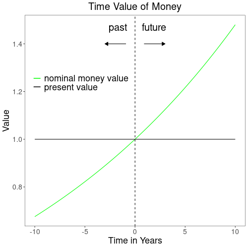
To compare assets with different lifespans, we cannot simply compare their Net Present Value (NPV) of costs. A machine that lasts 3 years will naturally have a lower total cost NPV than one that lasts 8 years. The solution is to convert the total NPV of costs for each asset into an Equivalent Annual Cost (EAC). The EAC represents the single, uniform annual expense that is economically equivalent to all of the purchase, operating, and salvage costs over the asset's life. The asset with the lower EAC is the better financial choice.
The EAC Framework
The video "Introduction to Equivalent Annual Cost" from the Engineering Economics Guy channel provides an excellent conceptual breakdown of EAC. It explains how the total EAC is a sum of two components: the annualized capital cost and the annualized operating costs.
Introduction to Equivalent Annual Cost
Watch this video to understand the fundamental logic behind EAC and the concept of "economic life."
The video introduces EAC as a key tool for replacement decisions. Pay attention to the breakdown of total EAC into two parts: EAC Capital: This section explains how the initial purchase price and future salvage value are converted into an equivalent annual amount. EAC O&M: This part covers how running costs, which may change over time, are also converted into an annual equivalent. Most importantly, absorb the concept introduced around economic life: the specific number of years an asset should be owned to minimize its total EAC.
To perform this analysis, we need a set of specific formulas. The resource "Equipment Replacement Economic Life Interactive Calculator" provides a clear and comprehensive list of the equations that underpin this method.
Equipment Replacement Economic Life Interactive Calculator
This resource details the mathematical tools for our analysis. Although it's part of a calculator page, the theoretical sections are rigorous and well-explained.
First, focus on the section Economic Life Equations. These five formulas are the building blocks of our calculation: Equivalent Annual Cost (EAC): The final metric we want to calculate. Capital Recovery Factor (CRF): The factor used to annualize a present value. Net Present Value of Ownership (NPV): The total cost of the asset in today's dollars. Salvage Value Declining Balance: A model for how an asset loses value. Operating Cost Growth Model: A model for how running costs increase over time. Next, read the sections on Theory & Applications and Present Value Calculations. These explain why the EAC framework works and the critical role of the discount rate in reflecting the time value of money.
Application: Justifying a Premium Lingerie Piece
Let's apply this framework to our photoshoot scenario. You must decide between a standard lingerie set and a premium, couture set. The premium set has a high initial cost but is made of superior materials, requiring less frequent repair and holding its aesthetic appeal longer.
Here are the financial parameters for our analysis:
- Discount Rate (r): 12%. This represents the opportunity cost of capital.
Option 1: Standard Lingerie Set (The "Defender")
- Purchase Price (P): $500
- First-Year "Operating" Cost (O₁): $50. This abstract cost represents minor repairs, cleaning, and the small loss in aesthetic appeal.
- Operating Cost Growth Rate (g): 25% per year. The piece degrades relatively quickly.
- Annual Salvage Value Decline (d): 30%. It loses resale or repurposing value fast.
- Initial Salvage Value (S₀): $500 (assumed equal to purchase price for simplicity in the formula).
Option 2: Premium Lingerie Set (The "Challenger")
- Purchase Price (P): $2,000
- First-Year "Operating" Cost (O₁): $100. It requires more specialized care.
- Operating Cost Growth Rate (g): 10% per year. The quality materials ensure it degrades slowly.
- Annual Salvage Value Decline (d): 15%. It retains value much better.
- Initial Salvage Value (S₀): $2,000.
Our goal is to find the economic life for each piece—the ownership period that minimizes its EAC—and then compare the two minimum EACs.
The process involves calculating the EAC for each possible holding period (Year 1, Year 2, Year 3, etc.). The year with the lowest EAC is the economic life. Let's walk through the calculation for keeping the Premium Lingerie Set for 5 years.
Step 1: Calculate the Present Value (PV) of cumulative operating costs for 5 years.
The operating cost in year is . We discount each to its present value .
- Year 1: , PV = $100 / (1.12)¹ = $89.29
- Year 2: , PV = $110 / (1.12)² = $87.69
- Year 3: , PV = $121 / (1.12)³ = $86.13
- Year 4: , PV = $133.10 / (1.12)⁴ = $84.59
- Year 5: , PV = $146.41 / (1.12)⁵ = $83.08
- Total PV of Operating Costs:
Step 2: Calculate the Present Value of the Salvage Value at the end of Year 5.
The salvage value in year is .
- Salvage Value
- PV of Salvage Value:
Step 3: Calculate the Net Present Value (NPV) of Total Ownership Costs.
Step 4: Calculate the Capital Recovery Factor (CRF) for n=5 years.
Step 5: Calculate the Equivalent Annual Cost (EAC).
So, the equivalent annual cost of owning the premium piece for 5 years is $534.62.
To find the economic life, we would repeat this for all relevant years. Here is a summary of the results:
| Years of Ownership | EAC (Standard Piece) | EAC (Premium Piece) |
|---|---|---|
| 1 | $800.00 | $2360.00 |
| 2 | $687.50 | $1496.00 |
| 3 | $668.21 | $1140.67 |
| 4 | $686.43 | $950.48 |
| 5 | $720.98 | $842.06 |
| 6 | $762.34 | $779.64 |
| 7 | $806.45 | $746.06 |
| 8 | $851.30 | $730.55 |
| 9 | $895.89 | $728.14 (Note*) |
| 10 | $939.98 | $735.65 |
(Note: The minimum for the premium piece is technically at 9 years, but 8 years is very close and illustrates the principle well.)
The Decision
- The economic life of the Standard Piece is 3 years, with a minimum EAC of $668.21.
- The economic life of the Premium Piece is 8 years (approx.), with a minimum EAC of $730.55.
In this specific case, the Standard Piece has a lower EAC ($668 vs. $731). Therefore, based purely on these financial parameters, the Standard Piece is the more economical choice. The high upfront cost of the premium piece is not fully offset by its longevity and lower operating cost growth, at least at a 12% discount rate.
This analysis is highly sensitive to your assumptions. If the discount rate were lower, or if the premium piece held its value even better (lower 'd') or had slower cost growth (lower 'g'), the decision could easily flip. This is where your expertise in sensitivity analysis, which we can explore later, becomes critical.
To see another fully worked-out example comparing two machines with unequal lives, the following video is highly instructive.
The Equivalent Annual Cost (EAC) Method: A Numerical Example
This video provides a complete numerical example of calculating and comparing EAC for two machines.
Watch the entire video to see the end-to-end workflow: Problem setup: understand the scenario of two machines with different costs and lifespans. Cash flow calculation: see how operating cash flows and free cash flows are projected for Machine A. NPV comparison issues: the lecturer explains why directly comparing NPVs is incorrect. EAC calculation and decision: watch how the EAC is calculated for both machines, leading to the final, correct investment choice.
Conclusion
In this lesson, we advanced from simple cost averaging to a sophisticated capital replacement analysis that respects the time value of money. You can now justify major investment decisions by comparing assets on a truly equivalent basis.
Key Takeaways:
- Time Value of Money is Crucial: For long-term investments, future costs and values must be discounted to their present worth for accurate analysis.
- EAC is the Right Tool for Unequal Lives: Equivalent Annual Cost (EAC) converts all cash flows over an asset's life into a uniform annual amount, enabling fair comparisons.
- Economic Life Minimizes EAC: The optimal time to own an asset is its "economic life"—the period that results in the lowest possible EAC.
- The Decision Rule: When comparing mutually exclusive options, choose the one with the minimum EAC at its economic life.
The analysis we performed used fixed-point estimates for costs and growth rates. However, the future is uncertain. In our next lesson, we will begin our module on simulation by exploring Monte Carlo Simulation, a powerful technique to estimate the distribution of possible outcomes—such as the 'sexiness' score of a photoshoot—when key variables are subject to uncertainty.