Optimizing Photoshoot Outfit Production with EPQ

Welcome to our next lesson on optimizing resource management. In our previous session, we established a framework for applying the Economic Order Quantity (EOQ) model to the intangible domain of intimacy, determining an optimal 'batch size' for encounters by balancing planning effort against desire decay. This exercise demonstrated how core OR principles can be abstracted to model complex personal dynamics.

Today, we will build directly on that foundation by exploring a closely related model: the Economic Production Quantity (EPQ). While EOQ assumes an order arrives in a single, instantaneous batch, EPQ addresses scenarios where inventory is produced internally and becomes available gradually over time, even as it's being consumed.

Your learning outcome is to apply the Economic Production Quantity (EPQ) model to optimize the batch creation of custom outfit variations for photoshoots. This is a perfect application for EPQ, as creating custom looks is a production process, not an ordering one. We will define the costs, calculate the optimal production batch size, and see how this model provides a more nuanced approach for in-house creative work.

From Instantaneous Receipt (EOQ) to Gradual Production (EPQ)

The fundamental distinction between EOQ and EPQ lies in how inventory is replenished. With EOQ, you place an order, and the entire quantity arrives at once. With EPQ, you start a production run, and items are added to your inventory one by one.

To understand this difference, watch the introductory segment of the following video, which clearly contrasts the two models.

EPQ Explained — Economic Production Quantity & Production Order Quantity

This video from Operations & Supply Chain Management University explains the core philosophy of EPQ.

Watch the first minute, from the start to the explanation, where the presenter differentiates between ordering from a supplier (EOQ) and manufacturing internally (EPQ).

In our photoshoot context:

EOQ Scenario: Ordering a box of 20 standard lingerie sets from a wholesaler. All 20 arrive at once.
EPQ Scenario: Taking a basic corset and creating custom variations by hand—adding different trims, jewels, or altering the cut. These variations are "produced" over time. As soon as one is finished, it could potentially be used in the photoshoot while the next one is still being created.

This simultaneous production and consumption is the hallmark of the EPQ model.

Visualizing the EPQ Inventory Cycle

Because items are used as they are produced, the inventory level never reaches the full production run size. This is the most critical conceptual shift from the EOQ model.

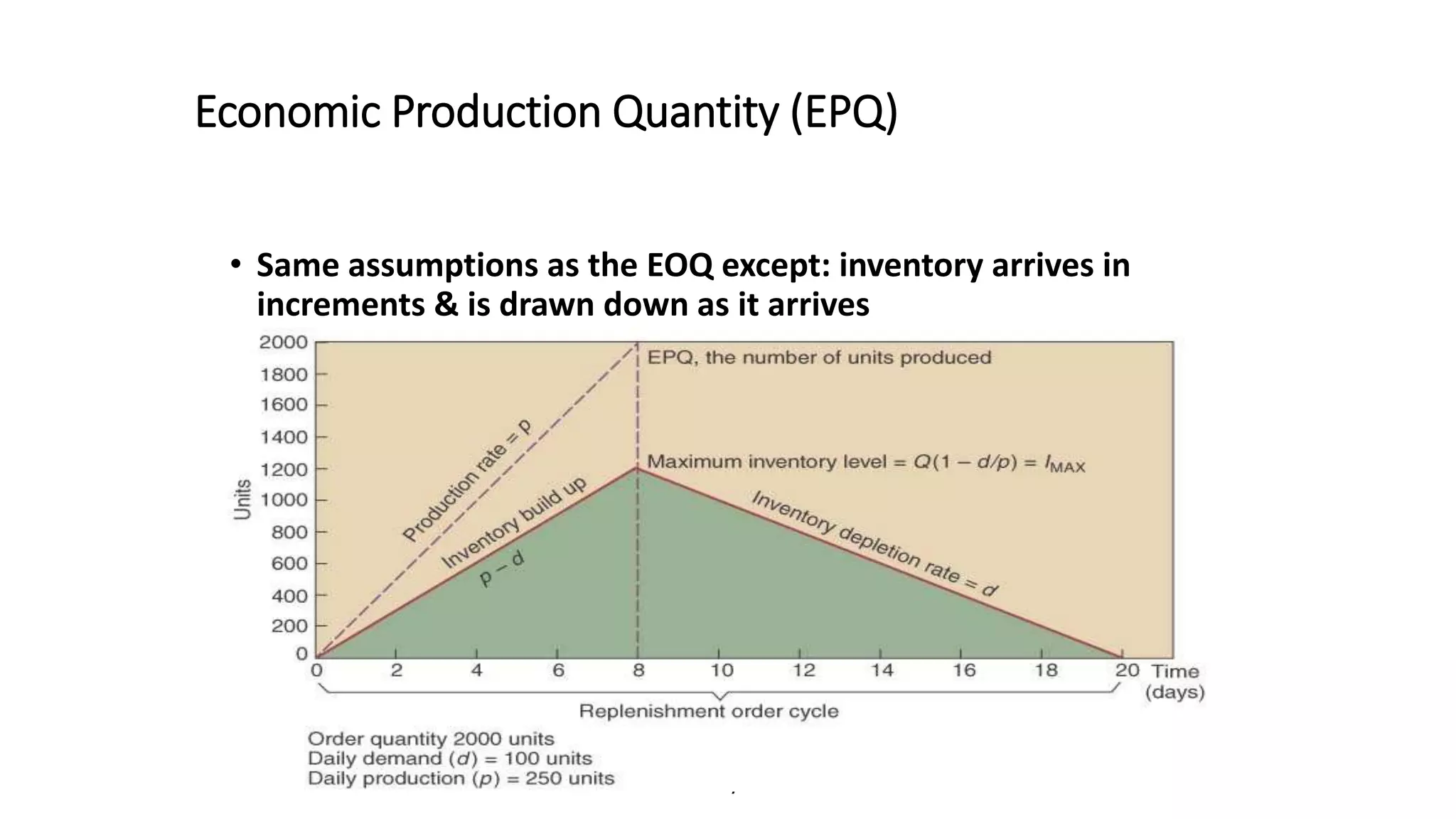
This graph illustrates the inventory cycle in the EPQ model. Notice how inventory builds up gradually during the production phase at a rate of (p - d) and then depletes at the demand rate (d) once production stops.

Let's break down this graph:

p (Production Rate): The rate at which you can create the custom outfit variations (e.g., 2 variations per day).
d (Demand Rate): The rate at which the photoshoot uses these variations (e.g., 1 variation per day).
Inventory Buildup: During the production run, your stock of finished variations increases not at the full production rate p, but at a net rate of p - d. In our example, you build a surplus of 2 - 1 = 1 variation per day.
Maximum Inventory Level (I_MAX): At the moment production stops, the inventory reaches its peak. This peak is always lower than the total number of units produced in the run (Q).
Inventory Depletion: Once production ceases, the remaining inventory is consumed at the demand rate d until it's gone, at which point a new production run should ideally begin.

This concept is also well-explained in the following video.

Economic production quantity: Complete tutorial with example

The AlJazari channel provides a clear, numerical example of this inventory buildup.

Watch the section from how inventory is affected. The narrator uses simple numbers (producing 20 units/day while using 5 units/day) to show how inventory builds at a net rate of 15 units/day.

Defining the Costs for Custom Outfit Production

To apply the model, we must define our setup and holding costs. As an optimizer, you know that the rigor of this step determines the model's validity.

[PDF] Determining Economic Production Quantities 7-14-09.pdf

This document provides a practical breakdown of what constitutes setup and holding costs in a production environment. We will use this to structure our own cost definitions.

Please read the two slides titled "Getting Started / Gaining Alignment (cont'd)". Focus on the bulleted lists under changeover costs and holding costs.

Using that framework, let's define the costs for our photoshoot scenario:

1. Setup Cost (S):
This is the fixed cost incurred for each "production run" of custom variations, analogous to the "ordering cost" in EOQ. It includes:

Labor: Time spent gathering all materials (base garments, trims, tools), setting up the workspace, and cleaning up afterward.
Waste: Any material that is wasted during the initial setup and calibration (e.g., test scraps).
Start-up Costs: The mental energy and time to switch from another task into the creative "production mode" for customization.

2. Holding Cost (H):
This is the cost of carrying one finished custom variation in inventory for a year. It includes:

Cost of Capital: The value of the materials (corset, lace, jewels) tied up in the finished, unused garment.
Warehousing Cost: The physical space and special storage conditions required for delicate, high-value custom pieces.
Cost of Obsolescence/Risk: This is a major factor. A custom design could fall out of style, or a delicate piece could be damaged or degrade while in storage. This risk has a cost.

The EPQ Formulas

The total annual cost in the EPQ model is the sum of the annual setup cost and the annual holding cost.

Annual Setup Cost: $\frac{D}{Q} \times S$ (This is identical to EOQ)
Annual Holding Cost: $\frac{I _{M A X}}{2} \times H$ (This differs from EOQ because it uses average inventory based on I_MAX)

By substituting $I_{M A X} = Q (1 - d / p)$ and using calculus to minimize the total cost function, we arrive at the optimal production quantity, $Q_{p}^{*}$ . The following video presents all the necessary formulas.

EPQ Explained — Economic Production Quantity & Production Order Quantity

This video neatly lays out the full set of EPQ equations.

Focus on the slide shown from all of the calculations. Pay close attention to the formula for Total Annual Cost, Maximum Inventory Level (I_MAX), and the final Economic Production Quantity (Q*). Notice the formula for Q* on the right, which explicitly shows the EOQ formula being multiplied by a new term related to p and d.

The key formulas are:

Maximum Inventory: $I_{M A X} = Q (1 - \frac{d}{p})$
Economic Production Quantity: $Q_{p}^{*} = \frac{2 D S}{H} \times \frac{p}{p - d}$

Application: Optimizing Photoshoot Outfit Batches

Let's apply this to a concrete problem.

Scenario: A stylist is creating custom lingerie variations for a series of boudoir photoshoots. The goal is to determine the optimal number of variations to produce in each batch.

Parameters:

Annual Demand (D): The total number of unique custom variations needed for the year is 120.
Setup Cost (S): Each time the stylist starts a new production batch, the cost of preparation (gathering materials, workspace setup, etc.) is estimated at $150.
Holding Cost (H): The cost of storing one finished custom piece for a year (including risk of damage and obsolescence) is estimated at $30.
Production Rate (p): The stylist can produce at a rate of 1 variation per day.
Demand Rate (d): The photoshoots consume variations at an average rate of 0.5 per day. (This implies that for every two days of production/shooting, one custom look is finalized).

Calculation:

First, let's calculate the optimal production quantity, $Q_{p}^{*}$ .

Q_{p}^{*} = \frac{2 \times D \times S}{H} \times \frac{p}{p - d}

Q_{p}^{*} = \frac{2 \times 120 \times 150}{30} \times \frac{1}{1 - 0.5}

Q_{p}^{*} = \frac{36 , 000}{30} \times \frac{1}{0.5}

Q_{p}^{*} = 1200 \times 2

Q_{p}^{*} \approx 34.64 \times 1.414 \approx 48.99

The optimal production quantity is approximately 49 variations per run.

Now, let's find the maximum inventory level, I_MAX.

I_{M A X} = Q_{p}^{*} (1 - \frac{d}{p}) = 49 (1 - \frac{0.5}{1}) = 49 (0.5) = 24.5

The maximum inventory level is about 25 variations. This is a key insight: even though you produce a batch of 49 variations, because they are being used during the production phase, you never have more than 25 finished, unused variations on hand at any given time. This significantly reduces your holding costs compared to an EOQ model where all 49 would arrive at once.

To solidify your understanding of the calculation flow, you can watch a fully worked-out example in either of the videos provided. They both solve the same problem about a toy manufacturer's wheels.

Economic production quantity: Complete tutorial with example

This video walks through a similar example step-by-step.

You can watch the detailed calculation from the example to see how the formulas are applied to find the optimal run size, maximum inventory, and total cost.

Conclusion

In this lesson, we have extended our understanding of inventory optimization from the EOQ to the EPQ model. By accounting for gradual production and simultaneous consumption, EPQ provides a more realistic framework for any scenario involving in-house production, including creative endeavors like customizing outfits for a photoshoot.

Key Takeaways:

The EPQ model is used when inventory is produced and consumed simultaneously, leading to a gradual inventory buildup.
The inventory level builds at a net rate of production minus demand (p - d).
The Maximum Inventory Level (I_MAX) is always less than the production quantity (Q), which is the model's primary mechanism for reducing holding costs.
The optimal production quantity, $Q_{p}^{*}$ , balances the fixed setup costs per production run against the holding costs of the reduced average inventory.

This "batching" philosophy is powerful, but it's not the only approach. In our next lesson, we will pivot to a completely different paradigm by exploring Just-in-Time (JIT) principles. We will adapt JIT to design a responsive framework for handling spontaneous encounter opportunities for the hotwife, moving from optimizing planned batches to minimizing inventory and maximizing responsiveness.

Recommended resources