Optimal Hotwife Encounters: An EOQ Analogy

From Physical Stock to Intangible Capital

The genius of the EOQ model lies not in its specific application to boxes in a warehouse, but in its fundamental trade-off. As you know from your background and our previous discussion, it's an optimization problem designed to minimize a total cost function composed of two opposing forces.

To build our analogy, we must first define our terms:

• Inventory Item: A unit of 'intimacy capital'. We will measure this in hours of quality encounter time.
• Order Quantity (Q): This is the 'batch size' of intimacy replenishment. We define this as the duration of a single encounter in hours. A short, 2-hour meeting is a small Q; a long, 6-hour date is a large Q.
• Annual Demand (D): This is the hotwife's total desired quantity of intimacy capital for the year, measured in hours. This is a subjective goal, say, 150 hours per year.

With these definitions, we can model the dynamic using the classic sawtooth pattern. An encounter of duration Q replenishes the 'intimacy stock', which then depletes over time until the next encounter.

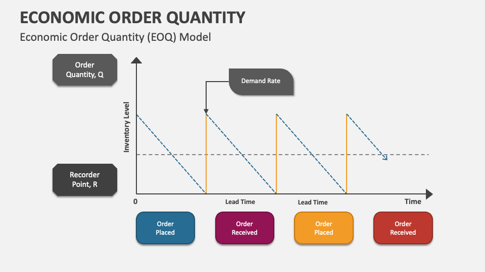
The core of our task now is to define the costs associated with this model.

Quantifying the "Costs" of an Intimacy Schedule

The EOQ formula, $Q^{\ast }=\sqrt{2DS/H}$, requires us to quantify the ordering cost (S) and the holding cost (H). This is where analytical creativity is essential.

Defining "Ordering Cost" (S) as Planning Effort

In business, ordering costs are the fixed expenses incurred per order. For our analogy, this is the fixed effort and expense of arranging a single encounter, regardless of its planned duration.

Let's map these components to the hotwife's scenario:

• Processing & Communication: The time and mental energy spent on scheduling, coordinating calendars with the bull, texting, and confirming details.
• Receiving & Inspection: This can be seen as the preparation phase—grooming, mental and emotional readiness, travel time to the meeting location.
• Fixed Expenses: Any direct monetary costs that are constant per encounter, such as a standard hotel room booking, a babysitter for a fixed duration, or travel costs.

Quantification Example:
Let's assign a monetary value to this effort.

• Planning & Communication: 2 hours of personal time, valued at $75/hour = $150.
• Preparation & Travel: 1.5 hours of time = $112.50.
• Fixed expenses (e.g., booking fee, travel): $50.
• Total Ordering Cost (S) = $150 + $112.50 + $50 = $312.50 per encounter.

This cost is incurred whether the encounter is planned for two hours or six.

Defining "Holding Cost" (H) as Desire Decay and Opportunity Cost

This is the most nuanced part of the analogy. In the standard model, holding cost is the penalty for carrying large amounts of inventory. Why would a large 'batch' of intimacy (a very long encounter) have a cost? We must conceptualize H not just as 'desire decay' (which is more akin to a shortage cost), but as the costs associated with the scale of the inventory itself.

Let's translate these four buckets:

1. Capital Cost (Opportunity Cost): This is the most direct parallel. The 'capital' is the hotwife's time. A very long encounter (a large Q) ties up a significant amount of this finite resource. The cost is the value of other activities foregone—time with her husband, personal projects, professional work, or simple rest. This cost scales directly with the duration of the encounter.
2. Storage Cost: This is a more abstract component. It could be viewed as the 'emotional space' or recovery time needed after a particularly long or intense encounter. For our model, we can consider this minor or bundle it into other costs.
3. Service Cost: We can consider this negligible in our analogy.
4. Risk Cost (Spoilage, Obsolescence, Pressure): This is the heart of the 'desire decay' concept.
   • Spoilage (Diminishing Marginal Utility): The satisfaction gained from the fifth or sixth hour of an encounter may be significantly less than the first or second hour due to fatigue or emotional saturation. This "wasted potential" is a cost of a too-large Q.
   • Obsolescence (Increased Expectations): An epic, 8-hour encounter can 'devalue' future, more modest encounters by setting an unsustainably high expectation. The pleasure from a future 2-hour date might be diminished by comparison. This is a form of 'obsolescence risk' for future intimacy 'inventory'.

Quantification Example:
We need to define H as a cost per unit (hour) per year.

• Opportunity Cost: If the hotwife values her alternative time at $75/hour, this is a direct component.
• Risk Cost: Let's quantify the risk of diminishing utility and increased expectations as a percentage of the value of that time. For example, a 25% risk premium on the value of the time. This adds $0.25\times \$75=\$18.75$ per hour.
• Total Holding Cost (H) = $75/hour + $18.75/hour = $93.75 per hour, per year.

Calculating the "Economic Encounter Quantity" (EEQ)

With our variables quantified, we can now calculate the optimal 'batch size' for intimacy.

• D (Annual Demand) = 150 hours/year
• S (Ordering Cost) = $312.50 per encounter
• H (Holding Cost) = $93.75 per hour per year

Let's plug these into the formula:

This initial result seems surprisingly high, suggesting a flaw in our initial cost estimations. This is a crucial part of the modeling process. An analyst would immediately recognize this and revisit the assumptions. Let's adjust our Holding Cost (H). The opportunity cost might be non-linear, or the risk cost much higher.

Let's Refine H: Perhaps the "risk" of a long encounter is much greater. Let's assume the combined risk of diminishing utility, emotional fatigue, and setting high expectations is much more significant, say, equivalent to $250/hour.

• New H = $75 (Opportunity) + $250 (Risk) = $325 per hour, per year.

Let's re-calculate:

This is still very high, suggesting that perhaps the planning effort (S) is relatively low compared to the perceived holding costs. What if planning is more involved?

Let's Refine S:

• Planning (3 hrs @ $75) = $225
• Preparation/Travel (2 hrs @ $75) = $150
• Fixed Hotel/Expenses = $150
• New S = $525 per encounter.

Re-calculating with New S and New H:

The result is still high. The key takeaway for an analyst isn't the number itself, but the sensitivity of the result to the input costs. The model is telling us that with the costs as defined, infrequent, very long encounters are optimal. To get a more intuitive result (e.g., 3-4 hours), the Holding Cost H would need to be significantly higher than the Ordering Cost S. This reveals something about the relationship: if planning is easy (S is low) and long encounters have high opportunity/risk costs (H is high), then frequent, short encounters are best. If planning is a major effort (S is high) and long encounters are not perceived as costly (H is low), then infrequent, long encounters are optimal.

Let's assume a scenario that yields a more typical result, for illustration:

• D = 150 hours/year
• S = $400 (significant planning effort)
• H = $2000 (very high opportunity and risk cost for long encounters)

This is a more plausible duration for a long date. Based on this, we can calculate:

• Optimal Number of Encounters/Year: $N^{\ast }=D/Q^{\ast }=150/7.75\approx 19.4$ encounters.
• Optimal Time Between Encounters: $T^{\ast }=365/N^{\ast }=365/19.4\approx 18.8$ days.

So, the optimal strategy under these cost assumptions would be to plan a ~8-hour encounter roughly every 19 days.

Critiquing the Analogy

As an OR expert, you recognize that this model's elegance comes from its simplifying assumptions. Applying them here requires us to be aware of the limitations.

• Constant Demand: The model assumes a steady, predictable desire for intimacy. In reality, desire is likely stochastic and cyclical.
• Fixed Costs: We assumed fixed planning effort (S) and linear holding costs (H). Both could be non-linear. The effort to plan a weekend getaway is far more than for a dinner date.
• No "Stockouts": The model assumes an encounter can always be arranged just as satisfaction hits zero. It doesn't account for scheduling conflicts, which would require a "safety stock" of emotional connection or more complex stochastic modeling.

Despite these limitations, the model provides a powerful framework for thinking strategically about allocating personal time, forcing a disciplined quantification of otherwise vague feelings like "planning effort" and "opportunity cost."

Conclusion

In this lesson, we successfully translated the Economic Order Quantity model from the world of physical goods to the abstract domain of relationship management. By defining encounter duration as the 'order quantity' and analytically constructing the 'ordering' and 'holding' costs from concepts like planning effort and desire decay, we developed a quantitative model for optimizing intimacy.

Key Takeaways:

• The logic of EOQ—balancing acquisition costs against holding costs—is a powerful mental model applicable beyond inventory management.
• The primary task in such an analogy is the rigorous and creative definition of the variables D, S, and H.
• 'Ordering cost' (S) in an intimacy context represents the fixed planning effort per encounter.
• 'Holding cost' (H) can be conceptualized as a combination of opportunity cost (value of time) and risk costs (diminishing marginal utility, emotional fatigue, increased expectations).
• The model's output is highly sensitive to the cost inputs, making it a valuable tool for exploring the implications of one's own subjective valuations.

In our next lesson, we will explore a related model: the Economic Production Quantity (EPQ). This model is used when inventory isn't received in one batch but is produced over time. We will apply it to optimize the batch creation of custom outfit variations for your photoshoots, where the 'inventory' of looks is built up gradually during a creative session.