Chain Ladder Method for Claims Reserving

The Logic and Assumptions of the Chain Ladder Method

The chain ladder method is built on a simple yet powerful assumption: the patterns of claim development observed in the past will continue in the future. In more formal terms, it assumes that for any given development period, the proportional increase in cumulative losses is stable across all accident years.

This assumption is the linchpin of the method. To see it stated formally, you can refer to the paper "A practical guide to the use of the chain-ladder method."

As the reading highlights, this core assumption may be violated by changes in business operations, the legal environment, or the presence of unusually large claims. Recognizing these limitations is as important as learning the method itself. For now, we will proceed assuming the patterns are stable. Our task is to quantify these patterns and use them to "complete" the triangle.

The mechanism for this is the calculation of age-to-age factors, more commonly known as Loss Development Factors (LDFs). An LDF measures the growth in cumulative claims from one development period to the next.

Step 1: Calculate and Select Loss Development Factors (LDFs)

For a single accident year $i$, the LDF for the development period from $j-1$ to $j$ is simply the ratio of the cumulative losses at those two points in time:

where $C_{ij}$ is the cumulative claim amount for accident year $i$ at development year $j$.

Since our run-off triangle gives us historical LDFs for several accident years, we must select a single, representative LDF for each development period that we will use for our projections. This is a key step involving actuarial judgment. Common choices include:

• A simple average of the historical LDFs.
• A volume-weighted average, which gives more weight to years with larger claim volumes.
• An average of the most recent years, if we believe recent history is more representative.

The following video provides a practical demonstration of calculating these LDFs and selecting an appropriate average.

The selection of LDFs results in a single vector of factors, one for each development interval (e.g., 12-24 months, 24-36 months, etc.).

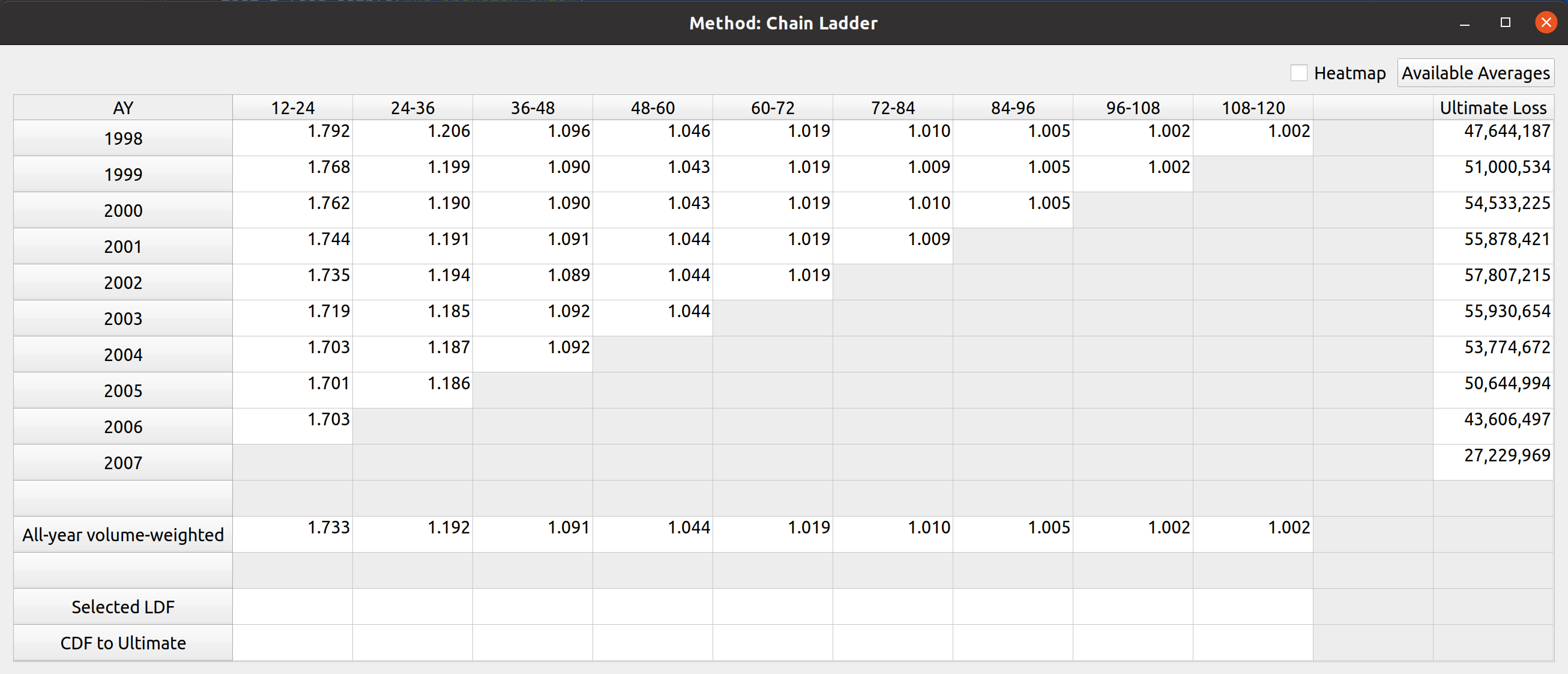
Step 2: Chain the Factors to Get Cumulative Development Factors (CDFs)

Once we have a selected LDF for each development interval, we can "chain" them together by multiplication to determine the total development from any given point to ultimate. This gives us the Cumulative Development Factor (CDF), or "factor-to-ultimate."

For example, the CDF to take claims from development year $j$ to their ultimate value is the product of all subsequent LDFs:

By convention, the LDF for the final development period is often assumed to be 1.000, meaning no further development is expected. This is called the "tail factor."

Let's return to the Mancinelli video to see this step.

Step 3: Project Ultimate Losses and Calculate Reserves

With the CDFs calculated, the final steps are straightforward:

1. Project Ultimate Losses: For each accident year $i$, multiply its latest observed cumulative loss, $C_{i,\text{latest}}$, by the corresponding CDF to project the ultimate loss, ${\hat{C}}_{i,\text{ult}}$.

   $${\hat{C}}_{i,\text{ult}}=C_{i,\text{latest}}\times {\text{CDF}}_{\text{latest}\to \text{ult}}$$

   The "latest" development period will be different for each accident year, corresponding to the values along the main diagonal of the triangle.

2. Calculate Outstanding Reserves: The outstanding reserve for each accident year is the difference between the projected ultimate loss and the cumulative loss reported to date. This is our estimate of the IBNR (which, in this context, stands for the total required reserve, including both pure IBNR and development on RBNS claims).

   $${\text{Reserve}}_i={\hat{C}}_{i,\text{ult}}-C_{i,\text{latest}}$$

3. Sum for Total Reserves: The total reserve liability is the sum of the reserves for all accident years.

   $$\text{Total Reserve}=\sum _i{\text{Reserve}}_i$$

This final part of the video demonstrates these last calculations.

A Complete Worked Example

To solidify your understanding, let's walk through a complete numerical example from start to finish. The following paper provides a clear, step-by-step application of the method.

This walkthrough provides a concrete example of the entire workflow, from the initial data to the final reserve figure, perfectly illustrating the application of the chain ladder method.

Conclusion

In this lesson, you have learned how to apply the basic chain ladder method, a cornerstone of actuarial reserving. By quantifying historical development patterns, you can make robust, data-driven estimates of future liabilities.

Key Takeaways:

• Core Assumption: The chain ladder method assumes that the proportional development of claims from one period to the next is consistent across accident years.
• Step 1: LDFs: Calculate historical age-to-age Loss Development Factors (LDFs) and select a representative factor for each development interval.
• Step 2: CDFs: "Chain" the selected LDFs together through multiplication to create Cumulative Development Factors (CDFs) that project losses to their ultimate value.
• Step 3: Reserves: Apply the CDFs to the latest cumulative losses to project ultimate losses. The reserve is the difference between the projected ultimate and the cumulative losses to date.

The basic chain ladder method is powerful in its simplicity, but its main assumption is not always valid. For example, what happens if claim costs are systematically increasing due to economic inflation? In that case, the development patterns of older years may not be representative of newer years. Our next lesson will address this exact problem by introducing the inflation-adjusted chain ladder method.