Introduction
In our last lesson, we mastered the basic chain ladder method, a cornerstone of actuarial reserving. We saw how to use historical claims data to project future liabilities under the core assumption that past development patterns will hold true for the future. However, as we briefly noted, this assumption can be fragile, especially in the face of economic forces like inflation.
This lesson tackles that very issue by introducing the inflation-adjusted chain ladder (IACL) method. We will learn how to refine the basic chain ladder approach to account for the systematic impact of inflation on claim amounts. Your background in statistics will be particularly useful here, as the process involves transforming the data to isolate a "pure" underlying pattern before making projections—a common technique in time series analysis. Our goal is to apply this more sophisticated method to a run-off triangle, calculate the reserves, and even incorporate discounting to find the present value of the liability.
Why Simple Projections Fail Under Inflation
The basic chain ladder method works with raw, nominal payment data. When inflation is present, this mixes two distinct effects:
- True Claim Development: The natural, operational pattern of how claims are reported and paid over time.
- Monetary Inflation: The general increase in the cost of goods and services, which inflates the monetary value of claim payments.
By treating a $100 payment from 2015 as equivalent to a $100 payment in 2022, the basic chain ladder method conflates these two effects. This distorts the calculated loss development factors (LDFs), as factors from older accident years (which contain lower-inflation payments) are averaged with those from newer years (with higher-inflation payments).
The IACL method solves this by systematically removing the effect of historical inflation before calculating development patterns, and then re-introducing expected future inflation into the projections. To get a high-level overview of this logic, the following article provides a concise explanation.
Claim Reserving Model Using the Chain-Ladder Method ... - Medium
This article by Ameya Damle on Medium clearly explains the rationale for incorporating inflation adjustments into the chain ladder method.
Please read the first three subsections: "Extending the Method," "Historical Inflation Adjustment," and "Future Inflation Projection." Focus on understanding the conceptual difference between adjusting past claims and projecting future ones.
As the article explains, the core idea is to bring all historical payments to a common price level (a "base year") before analysis. This allows us to isolate the true, underlying development pattern.
The Inflation-Adjusted Chain Ladder Method: A Step-by-Step Guide
The IACL method can be broken down into a logical sequence of steps. While it appears more complex than the basic method, it is simply a series of adjustments to purify the data before applying the familiar chain ladder logic.
The process is as follows:
- Create an Incremental Claims Triangle: Start with your cumulative claims triangle and calculate the incremental payments for each development period. The IACL method works directly with these individual payments.
- Deflate Historical Incremental Claims: Choose a base date (typically the most recent period, e.g., mid-2018). Using historical inflation rates, convert all past incremental payments to the price levels of this base date. This is done by dividing each payment by the appropriate cumulative inflation factor from its payment date to the base date.
- Form a Cumulative Inflation-Adjusted Triangle: Sum the deflated incremental claims to create a new cumulative claims triangle. The data in this triangle is now free of historical inflation effects.
- Calculate "Pure" LDFs: Apply the standard chain ladder technique to this new, inflation-adjusted cumulative triangle to calculate the LDFs. These factors now represent the development pattern without the distortion of inflation.
- Project Future Claims (at Base Prices): Use these LDFs to project the future claim payments and complete the inflation-adjusted triangle. The resulting projected incremental claims are still valued at the base date's price level.
- Inflate Future Incremental Claims: Take the projected incremental future payments (from the step above) and inflate them to their expected future payment dates using the assumed future inflation rates.
- Calculate the Reserve: The total reserve is the sum of these future, inflated incremental payments. If required, these payments can then be discounted to a present value using an assumed investment return rate.
Worked Example: IACL with Discounting
Let's apply this entire process to a typical exam-style problem. Your task is to calculate the discounted reserves based on the provided data.
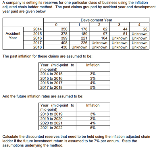
We will follow the steps outlined above. Our valuation date is the end of 2018, so we will use mid-2018 as our base period for pricing.
Step 1: Incremental Paid Claims Triangle
First, we convert the cumulative triangle into an incremental one by taking differences between adjacent development years.
| Accident Year | DY 0 | DY 1 | DY 2 | DY 3 | DY 4 |
|---|---|---|---|---|---|
| 2014 | 350 | 178 | 82 | 44 | 28 |
| 2015 | 378 | 189 | 97 | 51 | |
| 2016 | 399 | 221 | 104 | ||
| 2017 | 408 | 226 | |||
| 2018 | 430 |
Step 2: Deflate Historical Payments
We need to bring all payments to mid-2018 price levels. To do this, we first construct an inflation index with mid-2018 = 1.000.
- Index (mid-2018) = 1.000
- Index (mid-2017) = 1.000 / (1 + 5%) = 0.9524
- Index (mid-2016) = 0.9524 / (1 + 4%) = 0.9157
- Index (mid-2015) = 0.9157 / (1 + 3%) = 0.8891
- Index (mid-2014) = 0.8891 / (1 + 3%) = 0.8632
Now, we deflate each incremental payment by dividing it by the index corresponding to its payment year (Accident Year + Development Year). For example, the payment for AY 2014, DY 1, was made in 2015, so we divide it by the mid-2015 index.
Deflated Incremental Claims (at mid-2018 prices):
| Accident Year | DY 0 | DY 1 | DY 2 | DY 3 | DY 4 |
|---|---|---|---|---|---|
| 2014 | 405.47 | 200.21 | 89.54 | 46.20 | 28.00 |
| 2015 | 425.16 | 206.39 | 101.85 | 51.00 | |
| 2016 | 435.71 | 232.04 | 104.00 | ||
| 2017 | 428.40 | 237.33 | |||
| 2018 | 430.00 |
Step 3 & 4: Create Cumulative Adjusted Triangle and Calculate LDFs
We sum the deflated incremental claims to get the cumulative inflation-adjusted triangle. Then we calculate the volume-weighted LDFs from this triangle, just as we did in the basic chain ladder method.
Cumulative Inflation-Adjusted Claims:
| Accident Year | DY 0 | DY 1 | DY 2 | DY 3 | DY 4 |
|---|---|---|---|---|---|
| 2014 | 405.47 | 605.68 | 695.22 | 741.42 | 769.42 |
| 2015 | 425.16 | 631.55 | 733.40 | 784.40 | |
| 2016 | 435.71 | 667.75 | 771.75 | ||
| 2017 | 428.40 | 665.73 | |||
| 2018 | 430.00 |
LDF Calculation:
- LDF(0-1): (605.68 + 631.55 + 667.75 + 665.73) / (405.47 + 425.16 + 435.71 + 428.40) = 2570.71 / 1694.74 = 1.5169
- LDF(1-2): (695.22 + 733.40 + 771.75) / (605.68 + 631.55 + 667.75) = 2200.37 / 1904.98 = 1.1551
- LDF(2-3): (741.42 + 784.40) / (695.22 + 733.40) = 1525.82 / 1428.62 = 1.0680
- LDF(3-4): 769.42 / 741.42 = 1.0378
- LDF(4-ult): We assume a tail factor of 1.000 as no further development is given.
Step 5: Project Future Claims (at Base Prices)
We use the LDFs to project the future values along the diagonals of the cumulative adjusted triangle. For example, for AY 2018, the projected cumulative claim at DY 1 is .
Completed Cumulative Inflation-Adjusted Triangle:
| Accident Year | DY 0 | DY 1 | DY 2 | DY 3 | DY 4 | Ultimate |
|---|---|---|---|---|---|---|
| 2018 | 430.00 | 652.27 | 753.46 | 804.70 | 835.14 | 835.14 |
| 2017 | 428.40 | 665.73 | 769.01 | 821.28 | 852.36 | 852.36 |
| 2016 | 435.71 | 667.75 | 771.75 | 824.22 | 855.42 | 855.42 |
| 2015 | 425.16 | 631.55 | 733.40 | 784.40 | 814.07 | 814.07 |
| 2014 | 405.47 | 605.68 | 695.22 | 741.42 | 769.42 | 769.42 |
Step 6: Inflate Future Incremental Claims
By taking differences in the completed triangle, we find the projected incremental claims at mid-2018 prices. We must now inflate them to their actual payment dates.
- Future Inflation Index: We build an index for future payment dates, again relative to mid-2018=1.000.
- Index (mid-2019) = 1.000 * (1 + 3%) = 1.030
- Index (mid-2020) = 1.030 * (1 + 3%) = 1.061
- Index (mid-2021) = 1.061 * (1 + 4%) = 1.103
- Index (mid-2022) = 1.103 * (1 + 5%) = 1.159
The table below shows the projected incremental claims (at base prices), the year they are paid, the appropriate inflation factor, and the final inflated payment.
| AY | DY | Payment Year | Deflated Payment | Inflation Index | Inflated Payment |
|---|---|---|---|---|---|
| 2018 | 1 | 2019 | 222.27 | 1.030 | 228.94 |
| 2018 | 2 | 2020 | 101.19 | 1.061 | 107.36 |
| 2018 | 3 | 2021 | 51.24 | 1.103 | 56.52 |
| 2018 | 4 | 2022 | 30.44 | 1.159 | 35.28 |
| 2017 | 2 | 2019 | 103.28 | 1.030 | 106.38 |
| 2017 | 3 | 2020 | 52.27 | 1.061 | 55.46 |
| 2017 | 4 | 2021 | 31.08 | 1.103 | 34.28 |
| 2016 | 3 | 2019 | 52.47 | 1.030 | 54.04 |
| 2016 | 4 | 2020 | 31.20 | 1.061 | 33.10 |
| 2015 | 4 | 2019 | 29.67 | 1.030 | 30.56 |

Step 7: Calculate Discounted Reserves
The final step is to discount each future inflated payment back to the valuation date (end-2018). The payment in 2019 (mid-point) is 0.5 years away, the payment in 2020 is 1.5 years away, and so on.
The discount factor is where .
| Payment Year | Inflated Payment | Time (t) | Discount Factor | Discounted Payment |
|---|---|---|---|---|
| 2019 | 228.94 | 0.5 | 0.9665 | 221.28 |
| 2019 | 106.38 | 0.5 | 0.9665 | 102.82 |
| 2019 | 54.04 | 0.5 | 0.9665 | 52.23 |
| 2019 | 30.56 | 0.5 | 0.9665 | 29.54 |
| 2020 | 107.36 | 1.5 | 0.9036 | 97.02 |
| 2020 | 55.46 | 1.5 | 0.9036 | 50.11 |
| 2020 | 33.10 | 1.5 | 0.9036 | 29.91 |
| 2021 | 56.52 | 2.5 | 0.8445 | 47.72 |
| 2021 | 34.28 | 2.5 | 0.8445 | 28.95 |
| 2022 | 35.28 | 3.5 | 0.7892 | 27.84 |
| Total | 717.42 |
The total discounted reserve that needs to be held at the end of 2018 is 717.42.
Conclusion
In this lesson, we have significantly enhanced our reserving toolkit by incorporating inflation. The inflation-adjusted chain ladder method provides a more robust estimate of reserves when claim costs are changing due to economic factors. While the calculation is more involved, the underlying logic is a clear extension of the principles you have already learned.
Key Takeaways:
- Problem: The basic chain ladder method is distorted by inflation, as it mixes "pure" claim development with monetary effects.
- Solution: The IACL method follows a Deflate -> Project -> Inflate process.
- Deflate: Historical incremental claims are brought to a common base price level before analysis.
- Project: LDFs are calculated on this inflation-free data and used to project future claims, which are still at base prices.
- Inflate & Discount: These projected claims are then inflated to their future payment dates and can be discounted to a present value.
The chain ladder methods rely entirely on past claims data to project the future. But what if the data is sparse or unreliable, especially for new lines of business? Our next lesson will introduce the Bornhuetter-Ferguson method, which combines a data-driven approach like the chain ladder with an external, a priori estimate of ultimate losses.