Understanding Run-Off Triangles for Claims Reserving

The Purpose of Claims Reserving

Insurance operates on an "inverted production cycle." Unlike a manufacturer who knows the cost of a product before selling it, an insurer collects a premium upfront but only discovers the final cost of the policy over time, as claims are reported and paid. This creates a fundamental need to estimate future liabilities.

The delay between a claim-causing event (an "occurrence") and the final payment creates uncertainty. This process can be visualized as a timeline.

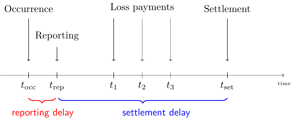
At any given moment (the "valuation date"), an insurer has a portfolio of claims at different stages:

• Closed Claims: The full cost is known and paid. No future liability exists.
• Reported But Not Settled (RBNS): The insurer knows about the claim, but future payments are still expected. The existing estimate for this is the case reserve.
• Incurred But Not Reported (IBNR): The event that will lead to a claim has happened, but the insurer is not yet aware of it. This is pure uncertainty.

The total claims reserve is the amount of money an insurer must set aside to cover all future payments for both RBNS and IBNR claims. This is one of the most significant liabilities on an insurer's balance sheet, and estimating it accurately is a core actuarial function.

To get a better handle on the key components that make up this total liability, let's watch a short video that breaks down the essential vocabulary.

To summarize the key relationships from the video:

• Incurred Loss = Paid Loss + Case Reserve
  • This represents the insurer's current estimate for known claims.
• Ultimate Loss = Incurred Loss + IBNR
  • This is the total final cost for all claims from a given period, including those not yet reported.
  • The IBNR portion itself includes two parts: "pure IBNR" (for claims not yet reported at all) and "IBNER" (Incurred But Not Enough Reported, meaning the case reserves for known claims are too low).

The goal of reserving is to estimate the Ultimate Loss for past periods, from which we can derive the required reserves.

The Structure of a Run-off Triangle

To estimate the ultimate loss, we need to organize historical claim data in a way that reveals patterns in how claims "develop" over time. We do this by aggregating the data from thousands of individual claims (micro-level data) into a specific tabular format called a run-off triangle (or development triangle).

A run-off triangle organizes claim data along three time dimensions.

Let's break down the structure:

1. Rows: Accident Year (or Occurrence Year)
   This is the year in which the event causing the claim occurred. All claims that happened in, say, 2020 are grouped together in the "2020 Accident Year" row, regardless of when they were reported or paid.

2. Columns: Development Year (or Age, Lag, Maturity)
   This represents the time elapsed since the beginning of the accident year. Development Year '0' is the accident year itself. Development Year '1' is the year after the accident year, and so on. A value in the column for Development Year '2' for the 2020 Accident Year row represents payments made during 2022 on claims that occurred in 2020.

3. Diagonals: Calendar Year (or Valuation Date)
   Each diagonal corresponds to a specific calendar year. For example, the values for (AY 2020, Dev 1), (AY 2019, Dev 2), and (AY 2018, Dev 3) all represent payments made during the calendar year 2021. The latest, most recent diagonal represents the data available at the current valuation date.

The combination of these axes gives the data its characteristic "triangle" shape, as we have more development history for older accident years than for more recent ones.

This next video provides a concise walkthrough of how to read the rows, columns, and diagonals of a loss triangle.

Incremental vs. Cumulative Data

The numbers within the triangle can represent different quantities. The two most common are:

• Incremental Claims: The amount paid (or reported) during that specific development period.
• Cumulative Claims: The total amount paid (or reported) up to the end of that development period.

The following resource provides clear examples of both formats.

Formal Notation

As a statistician, you will appreciate the formal notation used to describe the triangle. This notation is essential for defining the reserving problem mathematically.

Let:

• $i$ be the index for the accident year, from $i=1,\dots ,I$.
• $j$ be the index for the development year, from $j=0,\dots ,J$.
• $X_{ij}$ be the incremental claim amount for accident year $i$ in development year $j$.
• $C_{ij}$ be the cumulative claim amount for accident year $i$ as of the end of development year $j$.

The relationship is simple: $C_{ij}={\sum }_{k=0}^j{X}_{ik}$.

At a valuation date at the end of year $I$, we have observed all claim amounts $C_{ij}$ for which the calendar year of payment $i+j-1\le I-1$. This forms the upper-left part of the triangle. The reserving problem is to predict the values in the lower-right, unobserved part of the triangle to estimate the ultimate claim amount for each accident year, $C_{iJ}$.

A Practical View: Working with Triangles in R

To make these concepts more concrete, let's see how actuaries handle this data in a typical software environment like R. The ChainLadder package is a standard tool for this purpose.

The plots in the R example are particularly revealing. The plot of cumulative data typically shows a series of concave-down curves, where claims develop quickly in early years and then level off as they approach their ultimate value. This visual pattern is what allows us to build predictive models.

Conclusion

In this lesson, we have laid the crucial foundation for claims reserving. You now understand why it's necessary and how historical data is meticulously organized to facilitate the estimation of outstanding liabilities.

Key Takeaways:

• Purpose: Claims reserving is necessary because of the time lag between when a claim occurs and when it is finally settled. The goal is to estimate the funds needed to cover future payments on past claims, specifically for RBNS and IBNR claims.
• Structure: The run-off triangle is the primary data structure used.
  • Rows represent accident years.
  • Columns represent development years (time since the accident).
  • Diagonals represent calendar years (valuation dates).
• Data Types: Triangles can contain incremental data (amounts paid in a period) or cumulative data (amounts paid up to a period).
• The Problem: The reserving task is to use the observed "upper triangle" of data to predict the unobserved "lower triangle" and thereby estimate the ultimate cost for each accident year.

Now that we have a well-structured data set, our next lesson will introduce the most fundamental method used to fill in the missing half of the triangle: the basic chain ladder method. This technique uses the patterns of past development to project future development, allowing us to calculate our first estimate of outstanding claims reserves.